• article
• demo
• archive

@article{ipol.2011.cm_fds,
    title   = {{Finite Difference Schemes for MCM and AMSS}},
    author  = {Mondelli, Marco and Ciomaga, Adina},
    journal = {{Image Processing On Line}},
    volume  = {1},
    year    = {2011},
    doi     = {10.5201/ipol.2011.cm_fds},
}
% if your bibliography style doesn't support doi fields:
    note    = {\url{https://doi.org/10.5201/ipol.2011.cm_fds}}

Communicated by Antonin Chambolle
Demo edited by Jose-Luis Lisani

• Adina Ciomaga ciomaga@cmla.ens-cachan.fr, CMLA, ENS Cachan
• Marco Mondelli m.mondelli@sssup.it, SSSA, Pisa

Abstract

The two algorithms apply finite difference schemes respectively for Mean Curvature Motion and Affine Morphological Scale Space.

References

1. 1. Alvarez, F. Guichard, P.-L. Lions and J.-M. Morel, Axioms and fundamental equations of image processing, Arch. Rational Mech. Anal., 123 (1993), no. 3, 199--257, DOI: 10.1007/BF00375127;
2. 1. Alvarez, J.M. Morel, Formalization and computational aspects of image analysis, Acta Numer., 1994, 1--59, DOI: 10.1017/S0962492900002415;
3. L.Moisan, Modeling and Image Processing, course notes, 2005;
4. M.A. Grayson, The heat equation shrinks embedded plane curves to round points, J. Differential Geom., 26 (1987), no. 2, 285--314, http://projecteuclid.org/euclid.jdg/1214441371;
5. 1. Sapiro, A. Tannenbaum, On affine plane curve evolution, J. Funct. Anal. 119 (1994), no. 1, 79--120, DOI: 10.1006/jfan.1994.1004;
6. L.C. Evans, J. Spruck, Motion of level sets by mean curvature, J. Differential Geometry, 33 (1991), no. 3, 635--681, http://projecteuclid.org/euclid.jdg/1214446559;
7. 1. 1. Chen, Y. Giga, S. Goto, Uniqueness and existence of viscosity solutions of generalized mean curvature flow equations, Proc. Japan Acad. Ser. A Math. Sci. 65 (1989), no. 7, 207--210, DOI: 10.3792/pjaa.65.207;
8. 1. Froment, F. Guichard, L. Moisan, Megawave code available, 2001;
9. 1. Ciomaga, M. Mondelli, On the Finite Difference Schemes for Curvature Motions, Proceedings of International Student Conference on Pure and Applied Mathematics, 2010.

Overview

Alvarez et al. (ref. 1) characterized axiomatically all image multiscale theories and gave explicit formulas for the partial differential equations generated by scale spaces. They showed that all causal, local, isometric and contrast invariant scale spaces are given by curvature evolution equations of the type

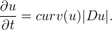
Two particular motions have become very popular for planar shape deformation and recognition algorithms. One refers to mean curvature flows

The other motion regards affine curvature evolutions

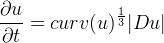
and is preferable to the Mean Curvature Motion for its projective invariance properties.

In the following we refer to algorithms based on finite difference schemes for computing mean and affine curvature evolutions of digital images, introduced by Alvarez and Morel (ref. 2). We discuss consistency, stability and convergence (for definitions see ref. 3). Our analysis focuses on some possible choices of the parameters, choices that generate multiple variants in the implementations. Meaningful visual examples on how the algorithms actually work are provided.

The algorithms run on both B/W and RGB images. When dealing with true color images, we perform the smoothing on each color channel independently.

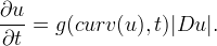
Mean Curvature Motion (MCM)

The Mean Curvature Motion has been studied in great detail for Jordan curves in a series of articles of differential geometry by Gage, Hamilton and Grayson (see for example ref. 4). In this classical setup, we are initially given a smooth Jordan curve and, as time progresses, we let each point evolve in the direction of the normal with a speed equal to the curvature at that point. It was shown that a curve instantly becomes smooth, shrinks asymptotically to a circle and shows no singularity or self-crossing.

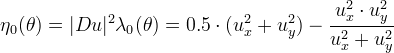
A completely different approach is given in the setting of viscosity solutions theory (see for example ref. 6,7), which provides rigorous mathematical justification for level set methods. The undertaking is analytically and numerically subtle principally because the mean curvature evolution equation is nonlinear, degenerate, and even undefined at points where Du=0. Indeed

Affine Morphological Scale Space (AMSS)

Affine curve evolution has been introduced by Sapiro and Tannenbaum (ref. 5). Together with Angenent, they gave existence and uniqueness proofs and showed a result similar to Grayson's theorem: a shape becomes convex and thereafter evolves towards an ellipse before collapsing. The viscosity solution theory developed by Chen, Giga and Goto (ref. 7) covers general curvature evolutions, including the AMSS.

It is worth mentioning that this equation is affine invariant in the sense that if we take a C² function u which is a solution of the AMSS, then

is also a solution, where A is a 2x2 matrix with positive determinant |A|.

Algorithms

Notations and Common Architecture

The program

• reads an image.tiff given as input
• checks if the image is true RGB
• applies a finite difference scheme for the Mean Curvature Motion at normalized scale R
• writes the result as a new image.tiff and returns it as output.

An image is false RGB if it has three identical color channels. In this case, only the array registered in the first channel is processed, the successive ones being discarded.

At normalized scale R every disk with radius less or equal than R disappears.

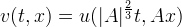
Finite Difference Scheme for MCM

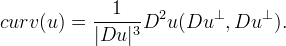
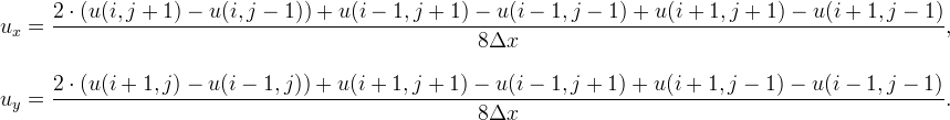
We consider a discrete image u(i,j) as an array of n_row x n_col integer samples taken from the continuous function u. The index i represents the current row number and j the current column number. We implement a finite difference scheme (FDS) taking advantage of the diffusive interpretation of the equation, i.e. the mean curvature can be expressed as the second derivative of u in the direction ξ orthogonal to the gradient

In fact

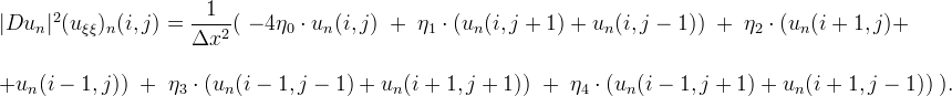
More precisely, we evaluate numerically u_ξξ with a linear scheme based on a 3x3 stencil and then we define iteratively the sequence u_n(i,j) by

To overcome the problem at points where the mean curvature evolution is undefined, we diffuse by half Laplacian whenever the gradient is below a threshold T_g (experimentally set to 4)

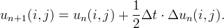
We point out that in practice, even if |Du|≠0 but too small in modulus, its direction becomes substantially random because it will be driven by rounding and approximation errors.

As suggested by Guichard, Morel and Ryan (ref. 2), if the gradient is not zero we can use a first neighborhood linear scheme for the evaluation of u_ξξ,

where Δx is the pixel width and will be set to 1.

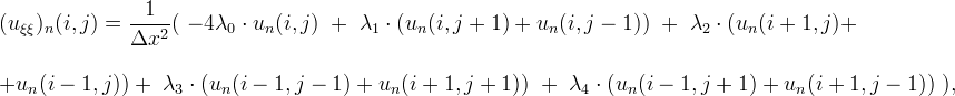
The formula can be rewritten in a more synthetic form, where ★ stands for a discrete convolution with a variable kernel A and θ is the angle between the gradient and the horizontal axis

We call A a variable kernel since the λ_i are not fixed, but depend on θ.

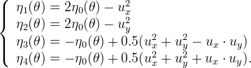
A simple Taylor development shows that in order to obtain consistency the following relationships must hold:

where sin θ and cos θ can be calculated from the following finite difference schemes of the partial derivatives of u,

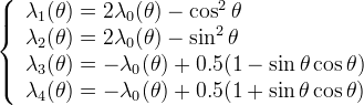
We have thus the value of λ₀ as the only free parameter, normally chosen to ensure stability. Such a condition implies that all λ_i must be positive. Unfortunately it is impossible to respect these inequalities except for particular values of θ, because

We decide to choose λ₀(θ) somewhere between the boundary functions so that λ₁ and λ₄ become only slightly negative.

The arithmetic mean of these two functions could be a valid candidate

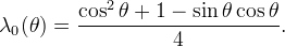
However our final decision is to take

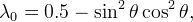
which is the trigonometric polynomial with least degree lying between boundary functions, smooth at 0 and π/4 and satisfying the following four geometrical requirements:

1. invariance by a rotation of angle π/2;
2. symmetry with respect to the axes i+j and i-j;
3. purely one-dimensional diffusion in the case θ=0;
4. purely one-dimensional diffusion in the case θ=π/4.

Finite Difference Scheme for AMSS

Following a procedure similar to that adopted for the MCM, we evaluate numerically the operator |Du|²u_ξξ with a linear scheme based on a 3x3 stencil and we define iteratively the sequence u_n(i,j) by

If the gradient is not zero we set

To ensure consistency η_i must satisfy

Instead a stability check is more difficult, because of the third root present in the equation defining the AMSS. So we limit to take simply

One would be tempted to choose for λ₀ the same value as for the MCM, but the arithmetic mean of boundary functions has the great advantage of being of degree 2.

This fact becomes important when we deal with the case |Du|=0, because differently from the MCM, the AMSS is well defined even when the gradient is zero,

Considering the numerical algorithm, we can see that η_i are well defined and no division by 0 is performed if and only if the degree of λ₀, thought as a trigonometric polynomial in θ, is less or equal than 2.

The results obtained after different choices of λ₀ and after the introduction of a threshold for the gradient will be compared in the next section.

MCM Implementations and Choice of the Parameters

The various implementations of a finite difference scheme for the Mean Curvature Motion can differ essentially on three aspects:

1. the way we deal with points situated on the edges of the image;
2. the way we overcome instability;
3. the choice of the time step.

A detailed analysis of these three points follows.

1. Image Extension

In order to apply a FDS to points situated on the borders, one needs to know the gray values of the pixels in the corresponding neighborhoods. However some of these neighbours could not be defined. In the continuous case we extend images by symmetry and periodization. Similarly, in the discrete case, an image can be extended by various procedures:

• mirror behavior: the discrete image is symmetrized with respect to x=0 and y=0;
• semi-mirror behavior: symmetry is performed with respect to x=0.5 and y=0.5;
• periodization;
• extension by 0 outside the image frame.

The origin is situated in the upper-left corner and the x-axis (respectively the y-axis) runs along the first row (respectively column).

We adopt the mirror behavior because it preserves the continuity of the image and avoids sharp changes at the edges. However, this choice has a major drawback: level lines meeting the frame of the image bend more and more as the scale increases. Actually, the image evolves as if it were the central block of a 9 times bigger image made up by 3x3 flips of the original one.

2. Instability

As pointed out before, the algorithm is not stable. Numerically, the maximum and minimum values assumed by the pixels exceed the range [0,255]. Nevertheless, in order to visualize the image it is necessary to restore pixel values to the original range. Basically there are four possibilities:

• saturation at the end: at the end of the iterative part we evaluate the maximum and minimum values assumed by the pixels and, if the case, set to 0 all the values below 0 and to 255 all the values above 255;

• saturation at each step: same operation as above, but performed after each single iteration;

• renormalization at the end: at the end of the iterative part we evaluate the maximum and minimum values assumed by the pixels. If they are not in the range, we apply an affine transformation T, such that

  

  An analytic expression for T in the first case is

  

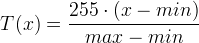
  and the other two cases can be easily reduced to the first one, taking respectively max=255 and min=0;

• saturation at each step: same operation as above, but performed after each single iteration.

The choice that allows us to remain attached to the original equation as much as possible is the first one. First of all renormalization is nothing but the application of a contrast change to all the pixels, while saturation modifies only the wrong ones, which are supposed to be in small number. Secondly, we prefer performing the operation when the iterative part is done to emphasize the fact that the problem is not algorithmical, but a matter of visualization. Moreover if the normalized scale is sufficiently high, in most cases the global maximum (minimum) after the initial increase (decrease) tends to return smaller than 255 (bigger than 0).

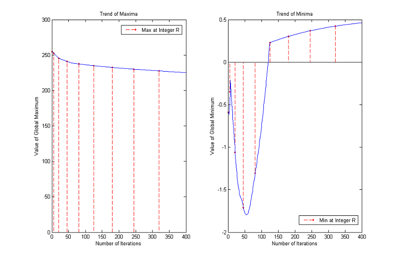
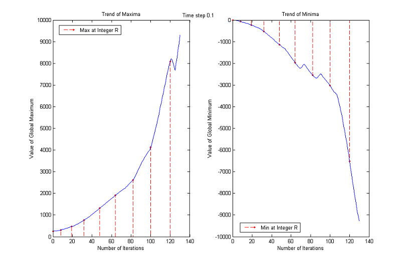
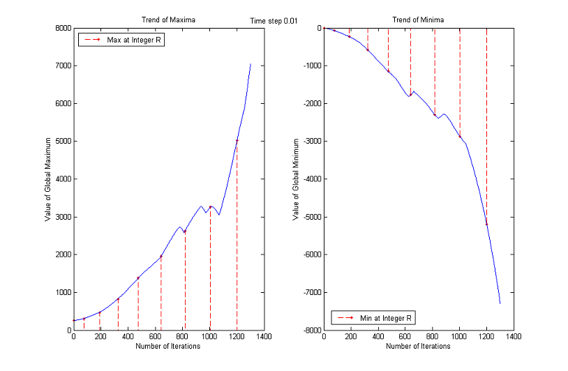
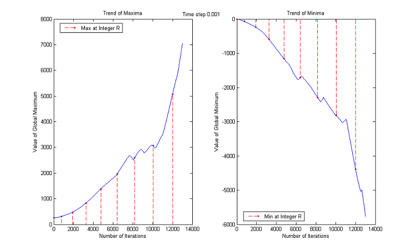
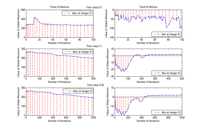
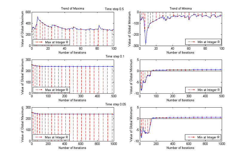
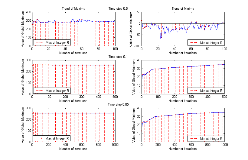
This behavior is testified by the following experiment. We took from the web some images at random and we plotted the maximum and minimum values assumed by the pixels after each iteration of the MCM for a total number of 400 (which means up to a normalized scale of almost 9). The numbers of iterations that correspond to integer normalized scales have been displayed in red, in order to be easily recognized.

For RGB images we evaluated the global maximum and minimum of the three arrays.

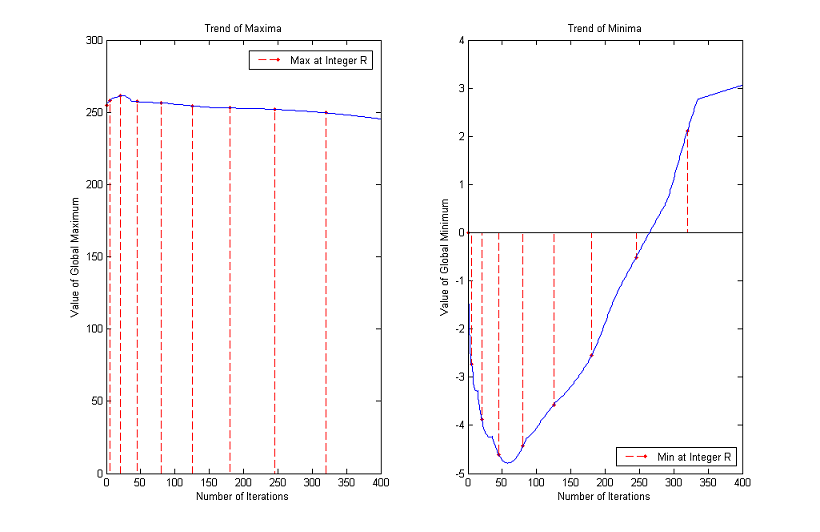
The maximum increases for the first 20 iterations (normalized scale about 2) and then decreases monotonically returning in range when we reach a normalized scale of about 5. The minimum stays below 0 much longer but at iteration 300 (normalized scale about 8) is again in the correct range.

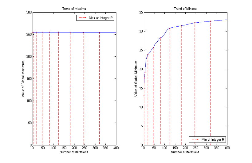
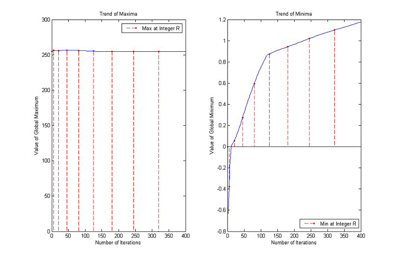
Trends of maxima and minima for other images

3. Time Step

The time step chosen for the experiments is Δt=0.1, but the results are about the same if Δt=0.5 or Δt=0.05, as the following comparative graphs clearly show:

More examples

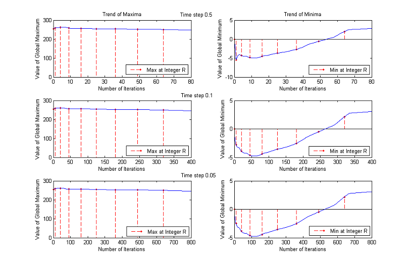
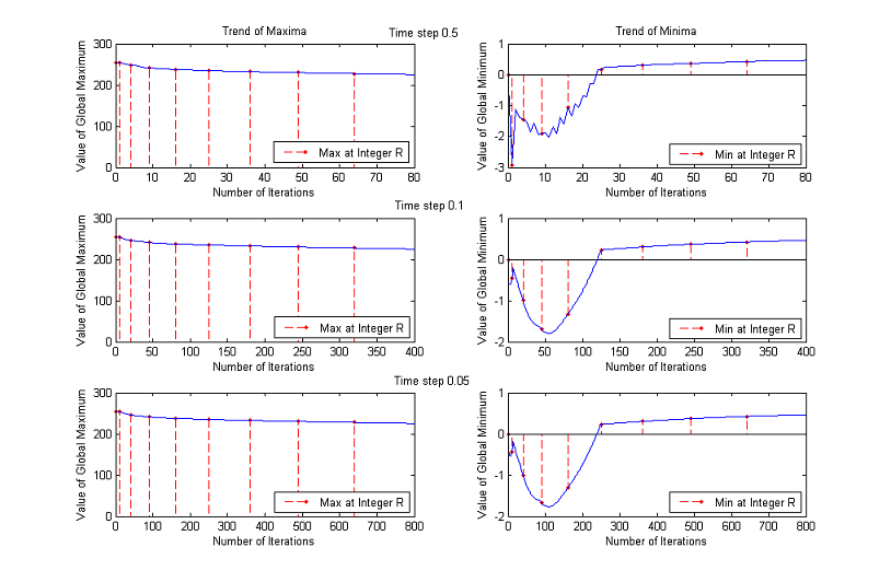
A good trade off between results and processing time is to set the value of time step to 0.1.

An upper bound for Δt is clearly 0.5, because of the application of the Heat Equation when the gradient is below the threshold, but performances are enhanced if we lower it further.

To decide the best value we performed two additional experiments, analyzing the results for Δt=0.5, Δt=0.1 and Δt=0.05.

Linear test

We checked if a linear function remains still after the application of the MCM.

An assessment test is to consider a linear image and to evaluate the difference between the original and its MCM evolution. The fewer the differences are, the better the algorithm is. We noticed that:

• different choices of the threshold for the gradient (T_g=1, T_g=2, T_g=4, T_g=8 and T_g=16) and different treatments of the pixels going outside the range [0,255] (renormalization/saturation at the end/at each step) produce identical results;
• if Δt=0.5, 84.7% of the pixels do not change after the application of the algorithm at a normalized scale of 5, while for Δt=0.1 or Δt=0.05 more than 98.7% of the pixels remains still.
• the two images processed with time steps respectively equal to 0.1 and 0.05 are identical; therefore it would be a waste of time to run the algorithm with Δt=0.05;
• when R increases the mirroring effect prevails, making the straight level lines bend.

Original image	MCM evolution of some level lines

Radial test

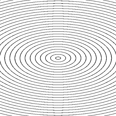
Similarly, we checked if a radial function remains still after the application of the MCM.

In this case the difference image is not useful, since we expect the level lines to remain circumferences, but to move. In practice we are interested in a numerical difference between the evolved level lines and real circles. The smaller the distance, the better the algorithm. To achieve this aim, we computed the difference between the maximum and minimum distance from the center of the image. The level lines too close to the edges were discarded since they would have been strongly deformed because of mirroring effect.

Ideally the difference should be zero, but such an eventuality does not occur even in the case of the original image. In fact the isolevel sets are not closed lines, but closed circular crowns of finite thickness, since there is an inevitable quantization operation when the image is written. The results follow:

• different choices of the threshold for the gradient and different treatments of the pixels out of the range produce identical output images;

• the best results are achieved with Δt=0.1;

• when R increases the difference between maximum and minimum distance also tends to grow, but not so much with respect to the initial value (which is a measure of the precision achievable with our radial check). We can notice considerable deformations of the level lines only when they are collapsing or if they are close to the boundaries of the image.

Original image	MCM evolution of some level lines

In conclusion, Δt=0.5 products the worst results, while the differences between the other two possibilities are not enough to make us decide for Δt=0.05, which will double the number of iterations and therefore processing time.

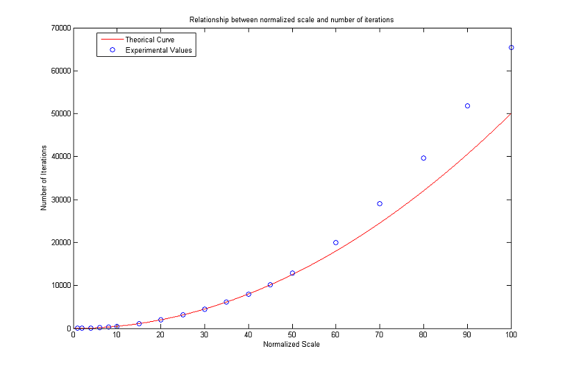
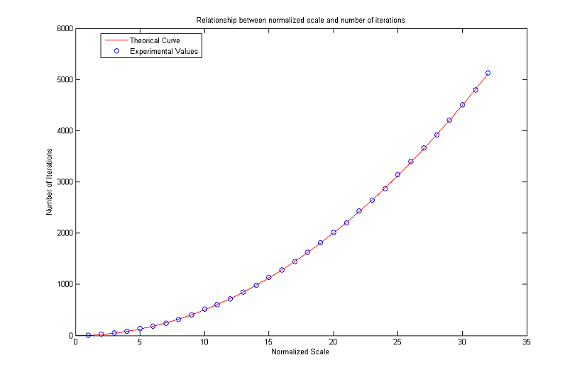
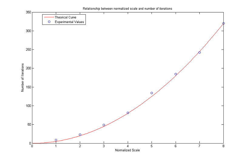
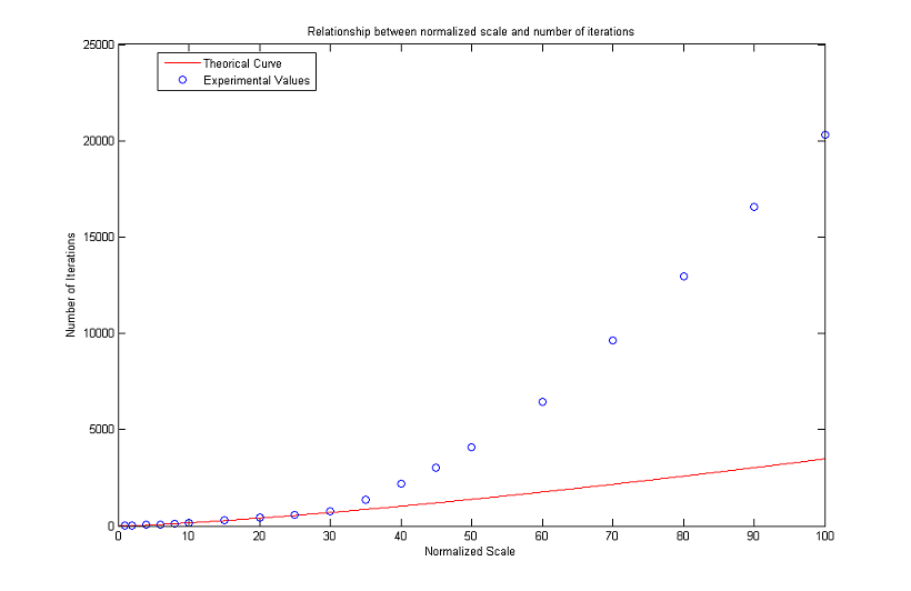
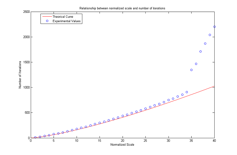
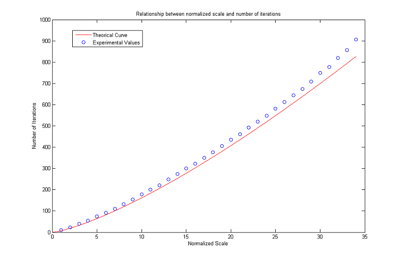
Relationship between Normalized Scale and Number of Iterations

We end the analysis regarding the MCM with a brief discussion on the relationship between normalized scale and number of iterations.

Our aim is to see how the formula

works out in practice.

To this end, we considered a digital image representing a circle (all the pixels whose distance from an assigned center is less or equal than the radius are black, the others are white). We then applied the algorithm until such a circle disappeared after a threshold with λ=127.5. This condition is satisfied when the gray value of the center (which is the global minimum) exceeds 127.5.

To minimize the mirroring effect we create bigger images as the radius of the circles increases: the number of rows (and therefore the number of columns, as the images are squares) is ten times the value of the radius and does not go below a minimum of 100. The results are plotted in the following figures. As can be seen, numerical values stay close to theoretical ones for normalized scales in [2, 50]. Then the curve of experimental values starts increasing faster and faster. The gap noticed for R low is probably due to the fact that the digital circles are not a good approximation of real circles because of pixelization, while the problems for high values of R are to be found in the finite difference scheme itself and limit the actual range of validity of the formula.

[Zoom In]

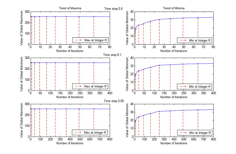
AMSS Implementations and Choice of the Parameters

Image extension and instability are treated similarly to MCM: we adopt a mirror behaviour with saturation at the end of the iterative part.

Stability

Setting

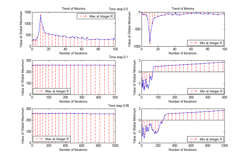
we remark that the global extrema blow up for any choice of time step, making the scheme unstable.

As before, we plot the trends of maxima and minima as functions of number of iterations until a normalized scale of almost 9. Red dashed lines connect the normalized scales to the corresponding maximum values.

[More time steps]

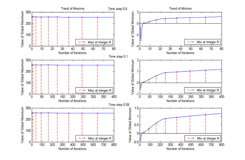
Instead, the other choice of λ₀ and consequently of η₀ make the algorithm almost stable.

In this way λ₀ is a trigonometric polynomial of degree 4, so we have to manage separately the case of zero gradient to avoid a division by 0.

Since

the first idea is to put a fictitious extremely low arithmetic threshold, say T_g=10^-6, and when the gradient is below it to take simply

However this solution is not consistent with the actual behavior of the continuous equation at the extrema: isolated extrema will not evolve and we know that is wrong, since small sets should collapse by curvature motion. To overcome the problem, we replace the AMSS with the Heat Equation when the gradient is too low.

Gradient Threshold

When making a choice of the threshold, we have to ensure two different tasks.

The application of finite difference schemes deals with floats, while for visualization we are obliged to adopt integer values. From a theoretical point of view, a continuous image is a smooth function from R² into R. To obtain the digital image we sample and round. Conversions from real to integer numbers yield rounding errors and make the direction of a gradient small in modulus substantially random. Nevertheless such approximation errors propagate only for the first iterations and then vanish because the whole iterative part is performed with a 4-bytes (float) precision. So eventually the threshold on the gradient is useful only to move isolated extrema.

Experimental data show that the way we pass from the initially higher value to the successive smaller one does not modify final results. So the on-line version presents T_g=4 for the very first iteration and T_g=1 for the following ones. Simple calculations show that the initial threshold T_g=4 implies an uncertainty in the evaluation of the gradient smaller than 15% in the worst case, while the value T_g=1 means that small sets will shrink to points in a reasonable number of iterations.

If we hadn't added such a geometrical threshold, the final validity check for the theoretical formula that links numbers of iterations with normalized scales would have been impossible.

Time Step

The tests were performed for Δt=0.5, Δt=0.1 and Δt=0.05 and concern stability, linearity, radiality (as previously presented) and ellipticity.

Stability

A first check allows to exclude immediately Δt=0.5, because this value makes the algorithm unstable.

We are considering ranges up to a normalized scale of 23, that is why we plot the first 100 iterations for Δt=0.5, the first 500 for Δt=0.1 and the first 1000 for Δt=0.05. Analyzing a wider range of numbers of iterations for Δt=0.5, we notice that the global maximum continues decreasing and that the values of the minimum oscillate remaining significantly below 0. The other two choices of time step instead yield similar results: for some images the maximum decreases monotonously, while for other ones remains close to the upper bound 255; the minimum, after the initial unstable behaviour, returns always bigger than 0.

More examples

Linearity and radiality

Different gradient thresholds and different treatments of the pixels going out of the range produce identical output images. As before, the optimal choice for time step is Δt=0.1 and, as can be seen in the graph below, AMSS preserves linearity and radiality better than MCM.

Ellipticity

Our aim is to verify that the evolved level lines are ellipses of constant axial ratio (equivalently, of constant eccentricity). In practice, due to quantization and pixelization isolevel sets are not ellipses but elliptical crowns. We are content with the numerical evaluation of the difference between the actual level lines and a real ellipse. To reduce the mirroring effect, for computations we considered only isolevel sets not too close to the boundaries of the image. Then we evaluated the major and minor axes, the focuses and the maximum and minimum sum of the distances between a generic point and the focuses. The difference between these two values is to be minimized.

As usual, different thresholds for the gradient and different treatments of the pixels out of the range produce the same output images. The best choice for the time step is Δt=0.05, but the improvement in performances with respect to the case Δt=0.1 is so small that makes us prefer Δt=0.1 for timing considerations. The axial ratio decreases slowly but almost monotonically, passing from the original value of 2 to 1.25 just before the isolevel set 20 disappears. The error on the distance remains quite close to the initial value of 4: unfortunately even for the initial image the accuracy in the detection of ellipses is scarce.

Original image	MCM evolution of some level lines

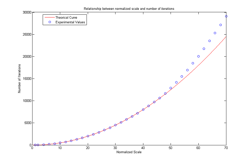
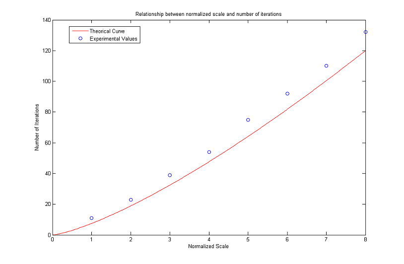
Relationship between Normalized Scale and Number of Iterations

As for the MCM, we complete our analysis with a discussion about the number of iterations versus the normalized scale. More precisely, we are interested in the range of values for which the following theoretical formula is valid in numerical simulations

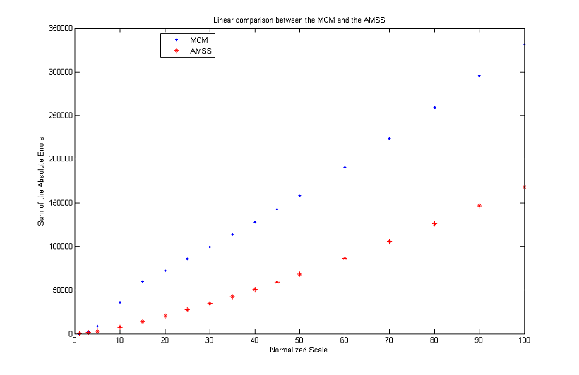
As can be seen in the following graphs, the approximation is reasonable until a normalized scale of about 34. Afterwards, the experimental values get further and further from the theoretical ones. For R low the problems are probably due to pixelization and scarce similarity between digital and analogical circles. However the results seem to be worse than the ones obtained for the MCM: for R in the range [10, 34] there is a percent error always higher than 5%, while for the MCM, if R is in the range [14, 46], then the percent error does not exceed 1%.

[Zoom In]

Online Demo

An online demo of the algorithms is available. The demo allows

• uploading an image (or using the default one);
• running the MCM and AMSS algorithms on the whole picture or on a zoomed detail;
• visualizing and comparing the results.

Source Code

An ANSI C implementation is provided: mcm, amss. The code is distributed under the license LGPL.

Source code documentation is also available: mcm, amss.

Examples

Remark: the normalized scale R is always given with respect to the original image. To find out the normalized scale for the zoomed detail, the value of R must be multiplied by the zooming factor.

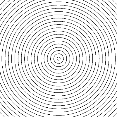
Geometrical Figures

Let's start our gallery with some examples taken from geometry. The MCM is applied at increasing integer normalized scales up to a maximum value of 10.

As expected, the corners gradually shrink becoming round and a fattening effect occurs between joint level sets.

[More on fattening effect]

In the following animation we apply the AMSS to a chessboard image until the middle squares disappear (R~34). This example also shows that the algorithm is not contrast invariant, which means that new gray levels can appear in the output image. The little gray shade then fattens conquering progressively almost all the space available.

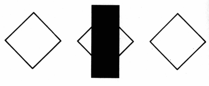
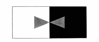
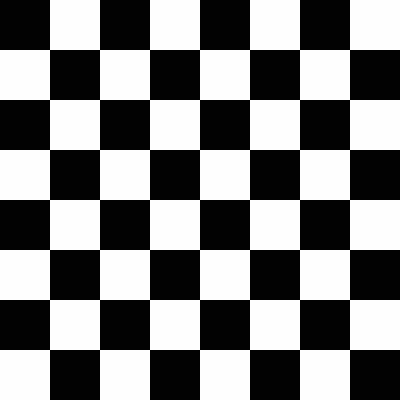
On the other hand, curves with thin boundary break and eventually collapse. This is a major drawback of pixel-based algorithms, which are limited to the initial grid and are blind to the intrinsic geometry of the image. A subpixel vision is required for accurate evolutions (see for example level lines shortening)

[More on disappearance of curves with small thickness]

Finite difference schemes are bad tools when dealing with such figures. In fact the thickness of the ellipse above is not big enough to create a black ribbon that can be evolved by the algorithm according to the theory. Generally speaking, making weighted means with the values of the first neighbours is a good idea when those values are continuously varying, but turns out to be highly problematic when handling black stripes on white backgrounds: if the majority of the neighbours are white, also the curve is going to turn white.

Graphs

We consider a 3x zoomed detail of one of the graphs analyzed before and we then apply the MCM and AMSS evolutions at normalized scale 1. Pixelization is eliminated and a visual improvement can be recognized, since the transition between colored parts and white background becomes smooth. The main drawback lies instead in the attenuation of shades, which makes the colors seem dull.

3x zoomed image	MCM evolution at scale 4/3	AMSS evolution at scale 4/3

Signs

In the following example, we have a look at the geometry of road signs.

From the original image below we extract a detail and we apply the MCM and the AMSS for R=1.

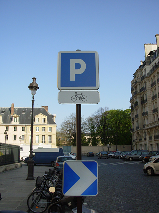
MCM/AMSS improve the quality of the image, because the pixelization effects disappear (see the corners of the P and especially the sketch representing the bike). The normalized scale has been chosen wisely because a higher value of R would have lead to the elimination of some particulars, such as the handle of the bicycle.

3x zoomed image	MCM evolution at scale 1	AMSS evolution at scale 1

[Truck ban]

For the original photo below, we zoom at first by a factor of 2 considering the whole sign and then by a factor of 6, focusing only on the truck ban.

The bigger writings are enhanced and we notice a real improvement, while the smaller ones in the lower part of the image appear attenuated. To obtain a better resolution one should zoom some more, discarding the rest of the sign.

2x zoomed image	MCM evolution at scale 1	AMSS evolution at scale 1

The reconstruction of the circular shape is good, but the lines that form the drawing of the bus are too thin to be satisfactorily managed by the algorithm.

6x zoomed image	MCM evolution at scale 2/3	AMSS evolution at scale 2/3

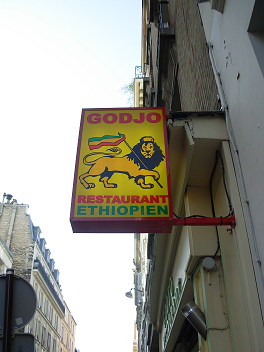
[Restaurant sign]

Pixelization effects are removed, the image becomes smoother and the result seems more natural to the human eye.

4x zoomed image	MCM evolution at scale 1/2	AMSS evolution at scale 1/2

[Information sign]

4x zoomed image	MCM evolution at scale 1/2	AMSS evolution at scale 1/2

JPEG Artifacts in Text and Handwriting

The well known JPEG coding is a commonly used method to compress images. Differently from TIF and PNG formats which are lossless, JPEG is lossy in the sense that after dividing the image in 8x8 pixel blocks and applying a discrete cosine transform (DCT), we make a quantization operation. In this way we lose inevitably some information, which from a visual point of view means artifacts, such as Gibbs's oscillations, staircase noise or checkerboarding. The MCM and the AMSS can be used to reduce these unwanted effects and actually yield a visual improvement if we zoom a specified part of the text.

2x zoomed image	MCM evolution at scale 1	AMSS evolution at scale 1

The results are even better in the following example, because the letters are spaced out enough. Nevertheless we pay the renewed smoothness of contours with a little bit of blurring.

3x zoomed image	MCM evolution at scale 4/3	AMSS evolution at scale 4/3

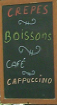
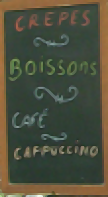
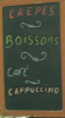
[Kiosk board]

The first three words can be read more easily in the evolved image, while the two P of "CAPPUCCINO" are too close and deform.

4x zoomed image	MCM evolution at scale 5/8	AMSS evolution at scale 5/8

Numberplates

Registration numbers need often preprocessing before applying recognition algorithms. MCM/AMSS smoothing might be one of the methods, though it does not always work well.

In the example below, the single letters do not mix up even if their borders seem to melt.

6x zoomed image	MCM evolution at scale 2/3	AMSS evolution at scale 2/3

[Indiscernible cases]

Nevertheless some letters are more readable than others. For example the fourth typeface of this numberplate is a Q. If a recognition is difficult in the first image, it is absolutely impossible to distinguish the Q from an O in the evolved pictures. In fact the short oblique stem that characterizes the letter shrinks after the application of the MCM/AMSS.

4x zoomed image	MCM evolution at scale 3/4	AMSS evolution at scale 3/4

Fingerprints

The usage of fingerprints for identification is more and more common nowadays.

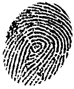
The application of the algorithm to this bad quality image allows us to restore the original smoothness of the fingerprint ridges.

3x zoomed image	MCM evolution at scale 4/3	AMSS evolution at scale 4/3

[Another example of fingerprints]

Here the quality of the image is a bit better, so we can try to apply a bigger zooming factor.

The contours appear more regular but the diffusion is too strong, due to oscillatory level sets. The gray shades that blur the image can be eliminated applying a threshold with λ=127.5 or adopting a stack filter. Both the operations will return as output a binary image.

5x zoomed image	MCM evolution at scale 1	AMSS evolution at scale 1

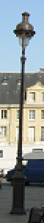
Lamps

Big particulars zoomed by a reasonable factor are easily handled by the algorithms, while, as the second example shows, dealing with small details in the background yields worse results. The blurring effect is considerable and evolved image is closer to an impressionist painting than to a real photo.

3x zoomed image	MCM evolution at scale 5/6	AMSS evolution at scale 5/6

3x zoomed image	MCM evolution at scale 2/3	AMSS evolution at scale 2/3

Leafy Branches

This particular of a tree, despite the small dimensions, contains a great amount of details and the calculation of curvatures is practically impossible. Diffusion prevails and the result is impressionistic.

However, as shown in the successive example, if the zooming factor and the amount of details considered reduce, an improvement in the quality of the image is still possible for twigs and leaves.

4x zoomed image	MCM evolution at scale 3/4	AMSS evolution at scale 3/4

3x zoomed image	MCM evolution at scale 2/3	AMSS evolution at scale 2/3

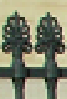
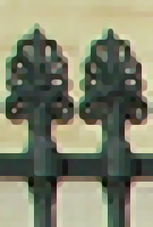
Fences

If with a 4x zoom we can still recognize acceptable output images, the successive 8x zoom is definitely too much for our finite difference schemes: the algorithms fail in identifying and enhancing the actual contours of the picture.

4x zoomed image	MCM evolution at scale 1/2	AMSS evolution at scale 1/2

8x zoomed image	MCM evolution at scale 3/8	AMSS evolution at scale 3/8

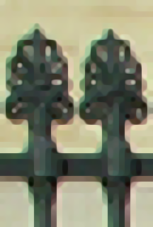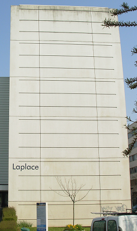
Buildings

Geometrical patterns representing contours can be restored by the MCM and the AMSS as long as the surrounding background does not have a complex structure.

6x zoomed image	MCM evolution at scale 5/6	AMSS evolution at scale 5/6

[Homogeneity gain]

As the normalized scale increases the color of facades gains in homogeneity and the horizontal lines tend to shrink.

6x zoomed image	MCM evolution at scale 1	AMSS evolution at scale 1