@article{ipol.2011.g_iics,
    title   = {{Image Interpolation with Contour Stencils}},
    author  = {Getreuer, Pascal},
    journal = {{Image Processing On Line}},
    volume  = {1},
    year    = {2011},
    doi     = {10.5201/ipol.2011.g_iics},
}
% if your bibliography style doesn't support doi fields:
    note    = {\url{http://dx.doi.org/10.5201/ipol.2011.g_iics}}
- published
- 2011-08-01
- reference
- Pascal Getreuer, Image Interpolation with Contour Stencils, Image Processing On Line, 1 (2011). http://dx.doi.org/10.5201/ipol.2011.g_iics
Communicated by François Malgouyres
Demo edited by Pascal Getreuer
- Pascal Getreuer
pascal.getreuer@cmla.ens-cachan.fr, CMLA, ENS Cachan
Overview
Image interpolation is the problem of increasing the resolution of an image. Linear methods have traditionally been preferred, for example, the popular bilinear and bicubic interpolations are linear methods. However, a linear method must compromise between artifacts like jagged edges, blurring, and overshoot (halo) artifacts. These artifacts cannot all be eliminated simultaneously while maintaining linearity.
More recent works consider nonlinear methods, especially to improve interpolation of edges and textures. An important aspect of nonlinear interpolation is accurate estimation of edge orientations. For this purpose we apply contour stencils, a new method for estimating the image contours based on total variation along curves. This estimation is then used to construct a fast edge-adaptive interpolation.
References
- F. Malgouyres and F. Guichard. “Edge direction preserving image zooming: A mathematical and numerical analysis.” SIAM J. Numerical Analysis, 39 (2002), pp. 1–37.
- D. Muresan. “Fast edge directed polynomial interpolation.” ICIP (2), 2005, pp. 990–993.
- A. Roussos and P. Maragos. “Reversible interpolation of vectorial images by an anisotropic diffusion-projection PDE.” Int. J. Comput. Vision, 2008.
- P. Getreuer. “Contour stencils for edge-adaptive image interpolation.” Proc. SPIE, vol. 7257, 2009.
- P. Getreuer. “Image zooming with contour stencils.” Proc. SPIE, vol. 7246, 2009.
- onOne software. “Genuine Fractals.” www.ononesoftware.com
Online Demo
An online demo of this algorithm is available.
Contour Stencils
The idea in contour stencils is to estimate the image contours by measuring the total variation of the image along curves. Define the total variation (TV) along curve C
![\|u\|_{\mathrm{TV}(C)} = \int_0^T \bigl|\tfrac{\partial}{\partial t}
u\bigl(\gamma(t)\bigr)\bigr| \,dt, \quad \gamma:[0,T]\rightarrow C](./g_iics_files/0fe6a5d1411ff341df8f97d73ccb97a7.png)
where γ is a smooth parameterization of C. The quantity ||u||TV(C) can be used to estimate the image contours. If ||u||TV(C) is small, it suggests that C is close a contour. The contour stencils strategy is to estimate the image contours by testing the TV along a set of candidate curves, the curves with small ||u||TV(C) are then identified as approximate contours.
Contour stencils are a discretization of TV along contours. As described in [4], [5], a ''contour stencil'' is a function 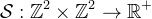 describing weighted edges between the pixels of v. Stencil
 ![]() is applied to v at pixel k ∈
is applied to v at pixel k ∈  as
as
![(\mathcal{S} \star [v])(k) :=
\sum_{m,n\in\mathbb{Z}^2}
\mathcal{S}(m,n) |v_{k+m} - v_{k+n}|.](./g_iics_files/117d7bcbf08239200d48de31734b3b87.png)
Defining [v](m,n) := |vm − vn|, this quantity is (with an abuse of notation) a cross-correlation over  evaluated at (k,k).
The stencil edges are used to approximate a curve C so that the quantity
evaluated at (k,k).
The stencil edges are used to approximate a curve C so that the quantity
![]() approximates ||u||TV(C+k) (where
C + k := {x+k : x ∈ C}). The image contours are estimated by finding a stencil with small TV. The best-fitting stencil at pixel k is
approximates ||u||TV(C+k) (where
C + k := {x+k : x ∈ C}). The image contours are estimated by finding a stencil with small TV. The best-fitting stencil at pixel k is
![\mathcal{S}^\star(k) =
\operatorname*{arg\,min}_{\mathcal{S}\in\Sigma}
(\mathcal{S} \star [v])(k)](./g_iics_files/d580ffb5ccc641c8710b238ef9ac487b.png)
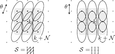
where Σ is a set of candidate stencils. It is possible that the minimizer is not unique, for example in a locally constant region of the image. For simplicity, we do not treat this situation specially and always choose a minimizer even if it is not unique. This best-fitting stencil ![]() provides a model of the image contours in the neighborhood of pixel k. The stencils used in this work are shown below.
provides a model of the image contours in the neighborhood of pixel k. The stencils used in this work are shown below.
The proposed stencil set Σ. The edge weights
For the set of candidate stencils Σ, we use 8 line-shaped stencils that were designed to distinguish between the functions

The edge weights α, β, δ, γ are selected so that on the function f(x) = x1sinθ − x2cosθ,
![|theta - pi/16 j| < pi/16 implies S^{pi/8 j} = argmin_{S in Sigma} (S star [f]).](./g_iics_files/e2ea77984a78391126946253d4810fdf.png)
In this way, the stencils can fairly distinguish 8 different orientations. An estimate of the local contour orientation at point k is obtained by noting which stencil is the best-fitting stencil ![]() .
.
 |
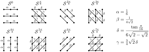
Normalized stencil total variations ![(\mathcal{S}^{\frac{\pi}{8}j} \star [f])](./g_iics_files/9be1da9a4086ad4423dacbdbe47a02e6.png) vs. θ. vs. θ.Left: The first three stencils, j = 0, 1, 2. Right: All eight stencils. |
For a color image, the image is converted from RGB to a luma+chroma space
![[Y U V]^T = [2 4 1; -1 -2 3; 4 -3 -1] * [R G B]^T](./g_iics_files/f3b465994042868157eb9caa621870ba.png)
and the stencil TV is computed as the sum of ![]() applied to each color channel.
applied to each color channel.
Interpolation
Given image v known on , we seek to construct an image u on  such that

where h is the (assumed known) point spread function and ∗ denotes convolution.
The goal is to incorporate deconvolution yet maintain computational efficiency. To achieve this, the global operation of deconvolution is approximated as a local one, such that pixels only interact within a small window.
Local Reconstructions
For every pixel k in the input image, we begin by forming a local reconstruction
where ![]() ⊂ is a neighborhood of the origin and
⊂ is a neighborhood of the origin and ![]() is a Gaussian oriented with the contour modeled by the best-fitting stencil
is a Gaussian oriented with the contour modeled by the best-fitting stencil ![]() .
.
Local reconstruction uk with oriented functions functions
The cn are chosen such that uk satisfies the discretization model locally,

This condition implies that the cn satisfy the linear system
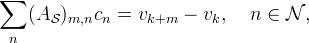
where ![]() is a matrix with elements
is a matrix with elements ![]() . By defining the functions
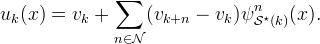
. By defining the functions
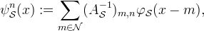
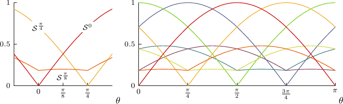
uk can be expressed directly in terms of the samples of v,
Global Reconstruction
The uk are combined with overlapping windows to produce the interpolated image,
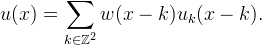
The window should satisfy ∑k w(x − k) = 1 for all x ∈ and w(k) = 0 for k ∈ \ ![]() .
.
Iterative Refinement
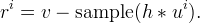
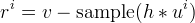
This global reconstruction satisfies the discretization model approximately,
↓(h ∗ u) ≈ v. The accuracy may be
improved using the method of iterative refinement.
Let ![]() denote the global reconstruction formula,
denote the global reconstruction formula,
![(\mathcal{R}v)(x) := \sum_{k\in\mathbb{Z}^2} w(x - k)\Bigl[
v_k + \sum_{n\in\mathcal{N}} (v_{k+n} - v_k) \psi^n_{\mathcal{S}^\star(k)}(x - k)
\Bigr]](./g_iics_files/2058218f80be505bda48e26c3efbce52.png)
such that u = ![]() v
(where we consider
v
(where we consider ![]() as fixed parameters
so that
as fixed parameters
so that ![]() is a linear operator).
Then the deconvolution accuracy is improved by the iteration
is a linear operator).
Then the deconvolution accuracy is improved by the iteration

Each iteration should reduce the residual in satisfying the discretization model,
The residual reduces quickly in practice, usually three or four iterations is sufficient for accurate results.
Parameters
The following parameters are fixed in the experiments:
- h is a Gaussian with standard deviation 0.5,
 = {-1,0,1}×{-1,0,1},
- w is the cubic B-spline,

 is an oriented Gaussian,

with στ = 1.2 and σν = 0.6, and θ is the orientation modeled by ,
,
and three iterations of iterative refinement are applied (one initial interpolation and two correction passes).
For sake of demonstration, the examples below use a PSF with a substantial amount of blur, σh = 0.5. The default value for σh is 0.35 in the online demo associated with this article, which better models the blurriness of typical images.
Algorithm
The interpolation is computationally efficient. We first consider the complexity without iterative refinement.
The matrices ![]() can be precomputed for each stencil
can be precomputed for each stencil ![]() ∈Σ, allowing the cn coefficients to be computed in 6
∈Σ, allowing the cn coefficients to be computed in 6![]() 2 + 3
2 + 3![]() operations per (color) input pixel. Furthermore, since w has
compact support, u only depends on the small number of uk where w(x − k) is nonzero. Let W be a bound on the number of nonzero terms,
operations per (color) input pixel. Furthermore, since w has
compact support, u only depends on the small number of uk where w(x − k) is nonzero. Let W be a bound on the number of nonzero terms,

We suppose that W is
O(![]() ).
Given the cn, each evaluation of u(x) costs
O(
).
Given the cn, each evaluation of u(x) costs
O(![]() 2)
operations. So for factor-d scaling, the
total computational cost is
O(
2)
operations. So for factor-d scaling, the
total computational cost is
O(![]() 2d2)
operations per input pixel.
For scaling by rational d, samples of w and
2d2)
operations per input pixel.
For scaling by rational d, samples of w and ![]() can also be
precomputed, and scaling costs
6
can also be
precomputed, and scaling costs
6![]() Wd2
operations per input pixel. For the settings used in
the examples, this is 864d2 operations per input pixel.
Wd2
operations per input pixel. For the settings used in
the examples, this is 864d2 operations per input pixel.
With iterative refinement, the previous cost is multiplied by the number of steps and there is the additional cost of computing the residual. If h is quickly decaying, then it is accurately approximated by an FIR filter with O(d2) taps and the residual
can be computed in O(d2) operations per input pixel.
Implementation
This software is distributed under the terms of the simplified BSD license.
- source code zip tar.gz
- online documentation
Please see the readme.html file or the online documentation for details.
Implementation notes:
- Fixed-point arithmetic is used to accelerate the main computations.
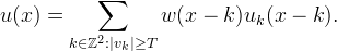
- For efficiency in the correction passes of iterative refinement, the uk for which |vk| is small are not added (so that they do not need to be computed),
Examples
Here we perform an interpolation experiment to test the performance of the proposed interpolation strategy.
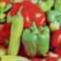
First, a high-resolution image uo is smoothed and downsampled by factor 4 to obtain a coarsened image v = ↓(h ∗ uo) where h is a Gaussian with standard deviation 0.5 in units of input pixels, σh = 0.5. This amount of smoothing is somewhat weak anti-aliasing, so the input data is slightly aliased.
The value of σh should estimate the blurriness of the PSF used to sample the input image. It is better to underestimate σh rather than overestimate: if σh is smaller than the true standard deviation of the PSF, the result is merely blurrier, but using σh slightly to large creates ripple artifacts.
The method works well for 0 ≤ σh ≤ 0.7. For σh above 0.7, the method produces visible ringing artifacts (even if the true PSF used to sample the input image has standard deviation σh). One could expect this effect, since there is no kind of regularization in the deconvolution. In the online demo, the default value for σh is 0.35, which reasonably models the blurriness of typical images.
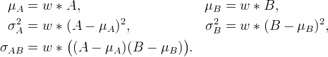
Interpolation is then performed on v to produce u approximating the original image uo. The interpolation and the original image are compared with the peak signal-to-noise ratio (PSNR) and mean structural similarity (MSSIM) metrics (How are these computed?).
 with each pixel represented by red, green, blue
intensities in
with each pixel represented by red, green, blue
intensities in  norms.
 ,
, ,
,
 ,
,
 .
.

Comparison with Other Methods
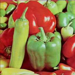
| Original Image (332×300) | Input Image (83×75) |
 |
 |
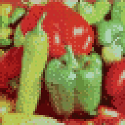
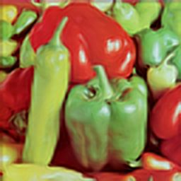
| Estimated Contour Orientations | Contour Stencil Interpolation PSNR 25.77, MSSIM 0.7165, CPU time 0.109s |
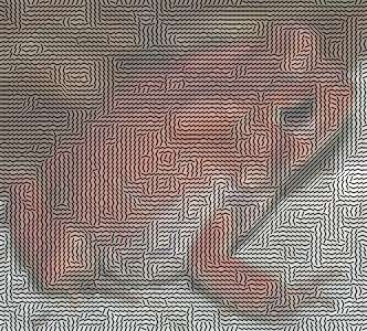 |
 |
The following table shows the convergence of the residual ri = v − ↓(h ∗ u) where the image intensity range is [0,1].
| Iteration i | ||ri||∞ |
| 1 | 0.05409007 |
| 2 | 0.01677390 |
| 3 | 0.00661765 |
For comparison, the same experiment is performed with standard bicubic interpolation, Muresan's AQua-2 edge-directed interpolation [2], Genuine Fractals fractal zooming [6], Fourier zero-padding with deconvolution, Malgouyres' TV minimization [1], and Roussos and Maragos' tensor-driven diffusion [3]. The first three of these methods do not take advantage of knowledge about the point spread function, while the later three do (notice their sharper appearance).
| Bicubic PSNR 24.36, MSSIM 0.6311, CPU time 0.012s |
AQua-2 [2] PSNR 23.97, MSSIM 0.6062, CPU time 0.016s |
 |
 |
| Fractal Zooming [6] PSNR 24.50, MSSIM 0.6317 |
Fourier Zero-Padding with Deconvolution PSNR 25.70, MSSIM 0.7104, CPU time 0.049s |
 |
 |
| TV Minimization [1] PSNR 25.87, MSSIM 0.7181, CPU Time 2.72s |
Tensor-Driven Diffusion [3] PSNR 26.00, MSSIM 0.7297, CPU Time 5.11s |
 |
 |
The contour stencil interpolation has good quality similar to tensor-driven diffusion but with an order magnitude lower computation time.
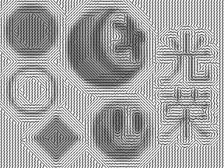
Geometric Features
The following experiment on a synthetic image tests the method's ability to handle different geometric features.
| Original Image (320×240) | Input Image (80×60) |
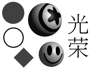 |
 |
| Estimated Contour Orientations | Contour Stencil Interpolation PSNR 21.23, MSSIM 0.8548, CPU time 0.078s |
 |
 |
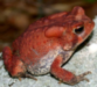
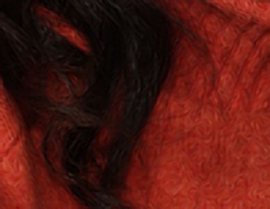
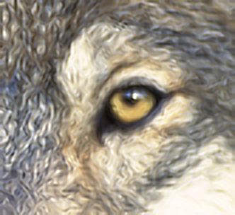
Textures
Because the method is sensitive to the image contours, oriented textures like hair can be reconstructed to some extent. Interpolation of rough textures with turbulent contours is less successful.
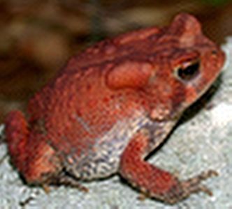
| Original Image (392×304) | Original Image (332×304) |
 |
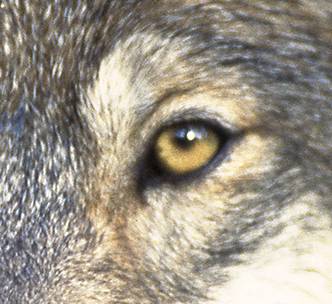 |
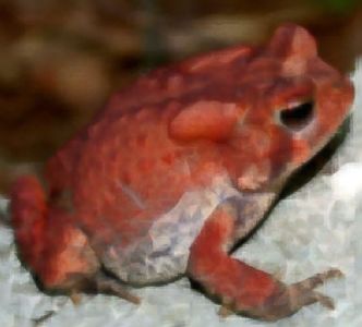
| Input Image (98×76) | Input Image (83×76) |
 |
 |
| Contour Stencil Interpolation PSNR 33.24, MSSIM 0.7762, CPU time 0.129s |
Contour Stencil Interpolation PSNR 22.47, MSSIM 0.6051, CPU time 0.115s |
 |
 |
Noisy Images
A limitation of the method is the design assumption that noise in the input image is negligible. If noise is present, it is amplified by the deconvolution. The sensitivity to noise increases with the PSF standard deviation σh, which controls the deconvolution strength. Similarly, if σh is larger than the standard deviation of the true PSF that sampled the image, then the method produces significant oscillation artifacts because the deconvolution exaggerates the high frequencies.
| Original Image (256×256) |
 |
The top row shows the input images and the bottom row shows their interpolations.
| Clean Input | JPEG Compressed | Quantized Colors |
 |
 |
 |
| Contour Stencil Interpolation PSNR 26.48, MSSIM 0.8196 |
Contour Stencil Interpolation PSNR 20.38, MSSIM 0.5244 |
Contour Stencil Interpolation PSNR 18.30, MSSIM 0.3393 |
 |
 |
 |
This material is based upon work supported by the National Science Foundation under Award No. DMS-1004694. Any opinions, findings, and conclusions or recommendations expressed in this material are those of the author(s) and do not necessarily reflect the views of the National Science Foundation. Work partially supported by the MISS project of Centre National d'Etudes Spatiales, the Office of Naval Research under grant N00014-97-1-0839 and by the European Research Council, advanced grant “Twelve labours.”
John D. Willson, USGS Amphibian Research and Monitoring Initiative
Pascal Getreuer
Pascal Getreuer
Peppers standard test image
Gary Kramer, U.S. Fish and Wildlife Service


