DCT image denoising: a simple and effective image denoising algorithm

Guoshen Yu; Guillermo Sapiro

doi:10.5201/ipol.2011.ys-dct

Guoshen Yu, Guillermo Sapiro

→ BibTeX

@article{ipol.2011.ys-dct,
    title   = {{DCT image denoising: a simple and effective image denoising algorithm}},
    author  = {Yu, Guoshen and Sapiro, Guillermo},
    journal = {{Image Processing On Line}},
    volume  = {1},
    year    = {2011},
    doi     = {10.5201/ipol.2011.ys-dct},
}
% if your bibliography style doesn't support doi fields:
    note    = {\url{http://dx.doi.org/10.5201/ipol.2011.ys-dct}}

published: 2011-10-24
reference: Guoshen Yu, and Guillermo Sapiro, DCT image denoising: a simple and effective image denoising algorithm, Image Processing On Line, 1 (2011). http://dx.doi.org/10.5201/ipol.2011.ys-dct

Communicated by Bartomeu Coll
Demo edited by Jose-Luis Lisani

Guoshen Yu yu@cmap.polytechnique.fr
Guillermo Sapiro guille@umn.edu

Overview

Digital images are often contaminated by noise during the acquisition. Image denoising aims at attenuating the noise while retaining the image content. The topic has been intensively studied during the last two decades and numerous algorithms have been proposed and lead to brilliant success.

This work presents an image denoising algorithm, arguably the simplest among all the counterparts, but surprisingly effective. The algorithm exploits the image pixel correlation in the spacial dimension as well as in the color dimension. The color channels of an image are first decorrelated with a 3-point orthogonal transform. Each decorrelated channel is then denoised separately via local DCT (discrete cosine transform) thresholding: a channel is decomposed into sliding local patches, which are denoised by thresholding in the DCT domain, and then averaged and aggregated to reconstruct the channel. The denoised image is obtained from the denoised decorrelated channels by inverting the 3-point orthogonal transform.

This simple, robust and fast algorithm leads to image denoising results in the same ballpark as the state-of-the-arts. Due to its simplicity and excellent performance, this contribution can be considered in addition as a baseline for comparison and lower bound of performance for newly developed techniques.

References

D.L. Donoho, I.M. Johnstone "Ideal spatial adaptation by wavelet shrinkage". Biometrika, vol. 83, pp. 425-455, 1994. DOI: 10.1093/biomet/81.3.425
R.R. Coifman, D.L. Donoho "Translation-invariant de-noising". Wavelets and Statistics, Springer Lecture Notes in Statistics, vol. 103, pp. 125–150, New York: Springer-Verlag, 1995.
1. Yu, G. Sapiro, S. Mallat "Solving Inverse Problems with Piecewise Linear Estimators: From Gaussian Mixture Models to Structured Sparsity". Submitted, 2010. arXiv:1006.3056v1

Online Demo

Try this algorithm on your own images with the online demonstration.

Source Code

The DCT image denoising source code that allows you to try the algorithm on your machine is available. gz

Algorithm

Threshold Estimation and Sparse Signal Representation

A signal f ∈ ℜ^N

is contaminated by a noise w ∈ ℜ^N

that is often modeled as a zero-mean Gaussian process independent of f

$\mathbf{y} = \mathbf{f} + \mathbf{w}$ ,

where y ∈ ℜ^N

is the observed noisy signal. Signal denoising aims at estimating f

from y

Let Β = { φ_n }_{1 ≤ n ≤ N}

be an orthonormal basis, whose vectors φ_n ∈ C^N

satisfy

$\langle \mathbf{\varphi_m}, \mathbf{\varphi_n} \rangle = \left\{ \begin{array}{ll} 1, & \text{if } m = n \\ 0, & \text{otherwise}. \end{array} \right.$

A thresholding estimator projects the noisy signal to the basis, and reconstructs the denoised signal with the transform coefficients larger than the threshold T

$\tilde{\mathbf{f}} = \sum_{n=1}^N \rho_T ( \langle \mathbf{y}, \mathbf{\varphi_n} \rangle ) \mathbf{\varphi_n},$

where

$\rho_T (x)= \left\{ \begin{array}{ll} x, & \text{if } |x| > T \\ 0, & \text{otherwise} \end{array} \right.$

is a thresholding operator.

The mean square error (MSE) of the thresholding estimate can be written as

$E[\|\mathbf{f} - \tilde{\mathbf{f}}\|^2] = \sum_{n: |\langle \mathbf{y}, \mathbf{\varphi_n} \rangle| \leq T} |\langle \mathbf{f}, \mathbf{\varphi_n} \rangle|^2 + \sum_{n: |\langle \mathbf{y}, \mathbf{\varphi_n} \rangle| > T} \sigma_n^2,$

where σ² = E [ | ⟨ w, φ_n ⟩ |² ]

. The first and second terms are respectively the bias and variance of the estimate. When the noise is Gaussian white of variance σ²

, it follows directly that

$E[\|\mathbf{f} - \tilde{\mathbf{f}}\|^2] = \sum_{n: |\langle \mathbf{y}, \mathbf{\varphi_n} \rangle| \leq T} |\langle \mathbf{f}, \mathbf{\varphi_n} \rangle|^2 + \sigma^2 |\{n: |\langle \mathbf{y}, \mathbf{\varphi_n} \rangle| > T\}|,$

where |{ • }|

denotes the cardinal of the set { • }

. Donoho and Jonestone have shown that, with a threshold equal to σ √ 2 log_e N

, the MSE of the thresholding estimate is close to that of an oracle projector (see ref. 1).

An orthonormal basis { φ_n }_{1 ≤ n ≤ N}

gives a sparse signal representation of a signal f

if the signal energy after the basis change is concentrated in a few transformed coefficients, while the rest of the coefficients are zero, i.e., |{n: |⟨ f, φ_n ⟩| ≠ 0}| << N

. Thresholding in a sparse representation reduces the variance of the estimate without increasing the bias, therefore resulting in small MSE and better denoising estimate.

DCT Local Patch Denoising

It is well known that local Discrete Cosine Transform (DCT) basis, applied in the most popular image compression standard JPEG, gives sparse representations of local image patches. The next figure illustrates an 8 x 8

DCT basis.

DCT basis

The proposed denoising algorithm decomposes the image into local patches of size √ N = 16 x 16

, and denoises the patches with thresholding estimate in the DCT domain. The 16 x 16

DCT window leads to on average the best denoising results. While it gives similar performance as smaller window size when the noise level is low ( σ < 30

), when the noise level is high it outperforms significantly smaller window, the gain with respect to window size of 8 x 8

from on average 0.5 to 2 dB as σ

goes from 50 to 100. A window size larger than 16 x 16

does not bring further significant improvement. (In the code, patch size of 16 x 16

is set by default, and 8 x 8

is a user option.)

It has been shown that introducing translation invariance considerably improves the thresholding estimate in an orthonormal basis (see ref. 2). Following a common practice (see ref. 3), translation invariant DCT denoising is implemented by decomposing the image to sliding overlapping patches, calculating the DCT denoising in each patch, and then aggregating the denoised patches to the image averaging the overlapped pixels. The translation invariant DCT denoising significantly improves the denoising performance, typically from about 2 to 5 dB, and removes the block artifact, at a cost of √ N x √ N

times calculation with respect to estimation with non-overlapping patches.

Color Decorrelation

The three color channels of a color image are typically highly correlated. Decorrelating the color channels before thresholding considerably improves the denoising estimate. To better understand this, let us take a sparse signal representation point of view and look at an extreme example where the three channels of an image are identical. Decorrelating the three channels at each pixel may produce a sparse signal representation with one non-zero coefficient out of three. A thresholding estimation thus reduces the noise variance to one third, which is equivalent to a PSNR improvement as high as 10 log₁₀(3) ≈ 4.7 dB

, orders of magnitude larger than some gain that most denoising algorithms struggle to achieve in a single image channel.

An orthonormal basis

$\{[1/\sqrt{3},~1/\sqrt{3},~1/\sqrt{3}]^T, [1/\sqrt{2},~0,~-1/\sqrt{2}]^T, [1/\sqrt{6},~-2/\sqrt{6},~1/\sqrt{6}]^T\}$

is used for color decorrelation. (Note that this is a 3-point DCT basis.) Each decorrelated color channel is then denoised separately by the DCT denoising algorithm described above. Comparing with standard color transformation such as the one from RGB to YUV, the orthonormal color decomposition slightly improves the denoising performance thanks to its orthogonality. The color decorrelation typically brings a PSNR improvement from about 1 to 3 dB.

Computational Complexity

The computational complexity of the DCT image denoising algorithm described above is dominated by that of the DCT transform of the patches.

A DCT transform of a one-dimensional signal of size N

can be implemented with a complexity O(N log N)

. A two-dimensional DCT transform on an image patch of size √ N x √ N

can be implemented in a separable way with a complexity O(N log √ N )

. An image of size S x C

, where S

is the number of pixels in each color channel and C

, typically equal to 3, is the number of color channels, contains S x C

sliding patches (slightly less than that in practice due to the border effect). The overall complexity is therefore O(SCN log √ N )

The DCT on different patches can be implemented in parallel, which may significantly reduce the computation time.

Implementation

Implemented in the C++ source file DCTdenoising.cpp.

Input: 
Noisy image
Gaussian white noise standard deviation: sigma
Output:
Denoised image

Algorithm:
If the image is colored, then decorrelate the color channels of the noisy image.
(C++ routine: ColorTransform)

Decompose each color channel to sliding patches.
(C++ routine: Image2Patches)

for each image patch
{
    Calculate 2D-DCT transform of the patch. (C++ routine: DCT2D)
    Threshold the DCT coefficients, with a threshold equal to 3sigma.
    Calculate inverse 2D-DCT transform of the patch. (C++ routine: DCT2D)
}

Average and aggregate the patches to reconstruct each denoised channel.
(C++ routine: Patches2Image)

If the image is colored, then reverse the color decorrelation to obtain the denoised image from the denoised channels,
(C++ routine: ColorTransform)
otherwise the denoised channel gives the denoised gray-level image.

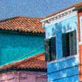
Examples

The following example illustrates the effectiveness of the DCT denoising algorithm. The noise is removed while the underlying image structures are preserved.

Original	Noisy, standard deviation 15	Denoised

Original (zoom)	Noisy, standard deviation 15 (zoom)	Denoised (zoom)