@article{ipol.2011.bcm_nlm,
    title   = {{Non-Local Means Denoising}},
    author  = {Buades, Antoni and Coll, Bartomeu and Morel, Jean-Michel},
    journal = {{Image Processing On Line}},
    volume  = {1},
    year    = {2011},
    doi     = {10.5201/ipol.2011.bcm_nlm},
}
% if your bibliography style doesn't support doi fields:
    note    = {\url{http://dx.doi.org/10.5201/ipol.2011.bcm_nlm}}
- published
- 2011-09-13
- reference
- Antoni Buades, Bartomeu Coll, and Jean-Michel Morel, Non-Local Means Denoising, Image Processing On Line, 1 (2011). http://dx.doi.org/10.5201/ipol.2011.bcm_nlm
Communicated by Guoshen Yu
Demo edited by Miguel Colom
- Antoni Buades
toni.buades@uib.es, CNRS-Paris Descartes - Bartomeu Coll
tomeu.coll@uib.es, Universitat Illes Balears - Jean-Michel Morel
morel@cmla.ens-cachan.fr, CMLA, ENS-Cachan
Overview
In any digital image, the measurement of the three observed color values at each pixel is subject to some perturbations. These perturbations are due to the random nature of the photon counting process in each sensor. The noise can be amplified by digital corrections of the camera or by any image processing software. For example, tools removing blur from images or increasing the contrast enhance the noise.
The principle of the first denoising methods was quite simple: Replacing the color of a pixel with an average of the colors of nearby pixels. The variance law in probability theory ensures that if nine pixels are averaged, the noise standard deviation of the average is divided by three. Thus, if we can find for each pixel nine other pixels in the image with the same color (up to the fluctuations due to noise) one can divide the noise by three (and by four with 16 similar pixels, and so on). This looks promising, but where can these similar pixels be found?
The most similar pixels to a given pixel have no reason to be close at all. Think of the periodic patterns, or the elongated edges which appear in most images. It is therefore licit to scan a vast portion of the image in search of all the pixels that really resemble the pixel one wants to denoise. Denoising is then done by computing the average color of these most resembling pixels. The resemblance is evaluated by comparing a whole window around each pixel, and not just the color. This new filter is called non-local means and it writes
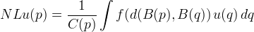
where d(B(p), B(q)) is an Euclidean distance between image patches centered respectively at p and q, f is a decreasing function and C(p) is the normalizing factor.
Since the search for similar pixels will be made in a larger neighborhood, but still locally, the name "non-local" is somewhat misleading. In fact Fourier methods for example are by far more nonlocal than NL-means. Nevertheless, the term is by now sanctified by usage and for that reason we shall keep it. The term "semi-local" would have been more appropriate, though. The implementation of the current online demo is based on a patch version of the original NL-means. This version is based in a simple observation. When computing the Euclidean distance d(B(p),B(q)), all pixels in the patch B(p) have the same importance, and therefore the weight f(d(B(p),B(q)) can be used to denoise all pixels in the patch B(p) and not only p.
For completeness, we shall give both the original (pixelwise) presentation, and the patchwise presentation of the same algorithm, which is somewhat more elegant.
References
- Buades, B. Coll, J.M. Morel
"A review of image denoising methods, with a new one"
Multiscale Modeling and Simulation, Vol. 4 (2), pp: 490-530, 2006. DOI: 10.1137/040616024
- Buades, B. Coll, J.M. Morel
"A review of image denoising methods, with a new one"
- Buades, B. Coll, J.M. Morel
"A non local algorithm for image denoising"
IEEE Computer Vision and Pattern Recognition 2005, Vol 2, pp: 60-65, 2005. DOI: 10.1109/CVPR.2005.38
- Buades, B. Coll, J.M. Morel
"A non local algorithm for image denoising"
- Buades, B. Coll, J.M. Morel "Image data processing method by reducing image noise, and camera integrating means for implementing said method", EP Patent 1,749,278 (Feb. 7), 2007.
Pixelwise Implementation
The denoising of a color image u=(u1, u2, u3) and a certain pixel p writes
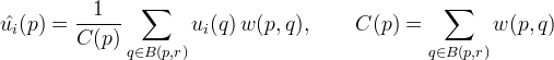
where i=1, 2, 3 and B(p, r) indicates a neighborhood centered at p and size 2r+1 × 2r+1 pixels. This research zone is limited to a square neighborhood of fixed size because of computation restrictions. This is a 21x21 window for small and moderate values of σ. The size of the research window is increased to 35x35 for large values of σ due to the necessity of finding more similar pixels to reduce further the noise.
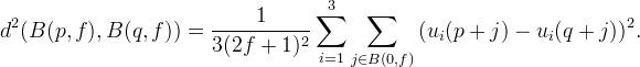
The weight w(p, q) depends on the squared Euclidean distance d² = d²(B(p,f), B(q,f)) of the 2f+1 × 2f+1 color patches centered respectively at p and q.
That is, each pixel value is restored as an average of the most resembling pixels, where this resemblance is computed in the color image. So for each pixel, each channel value is the result of the average of the same pixels.
We use an exponential kernel in order to compute the weights w(p, q)
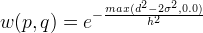
where σ denotes the standard deviation of the noise and h is the filtering parameter set depending on the value of σ. The weight function is set in order to average similar patches up to noise. That is, patches with square distances smaller than 2σ² are set to 1, while larger distances decrease rapidly accordingly to the exponential kernel.
The weight of the reference pixel p in the average is set to the maximum of the weights in the neighborhood B(p,r). This setting avoids the excessive weighting of the reference point in the average. Otherwise, w(p,p) should be equal to 1 and a larger value of h would be necessary to ensure the noise reduction. By applying the above averaging procedure we recover a denoised value at each pixel p.
Patchwise Implementation
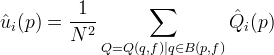
The denoising of a color image u=(u1, u2, u3) and a certain patch B = B(p,f) (centered at p and size 2f+1 x 2f+1) writes

where i=1, 2, 3, B(p, r) indicates a neighborhood centered at p and size 2r+1 × 2r+1 pixels and w(B(p,f),B(q,f)) has the same formulation than in the pixelwise implementation.
In this way, by applying the procedure for all patches in the image, we shall dispose of N² = (2f+1)² possible estimates for each pixel. These estimates can be finally averaged at each pixel location in order to build the final denoised image.
The main difference of both versions is the gain on PSNR by the patchwise implementation, due to the larger noise reduction of the final aggregation process. Spurious noise oscillations near edges are also reduced by the final aggregation process. However, the overall quality in terms of preservation of details is not improved by the patchwise version.
Parameters
The size of the patch and research window depend on the value of σ. When σ increases we need a larger patch to make patch comparison robust enough. At the same time, we need to increase the research window size to increase the noise removal capacity of the algorithm by finding more similar pixels.
The value of the filtering parameter writes h= k σ. The value of k decreases as the size of the patch increases. For larger sizes, the distance of two pure noise patches concentrates more around 2σ² and therefore a smaller value of k can be used for filtering.
Gray
|
Color
|
Source Code
Some of the files use algorithms possibly linked to the cited patent [3]. These files are made available for the exclusive aim of serving as scientific tool to verify the soundness and completeness of the algorithm description. Compilation, execution and redistribution of these files may violate exclusive patents rights in certain countries. The situation being different for every country and changing over time, it is your responsibility to determine which patent rights restrictions apply to you before you compile, use, modify, or redistribute these files.
The rest of files are distributed under GPL license. A C/C++ implementation is provided.
It should compile on any system since it's only strict ANSI C/C++ and is distributed under the GPL licence.
Basic compilation and usage instructions are included in the
README.txt file. This code requires
libpng and is limited to 8bit RGB or grayscale PNG image files.
The same code is used for the online demo.
On Line Demo: Try It!
An on-line demo of this algorithm is available.
The demo permits to upload any color image, add Gaussian noise and denoise it. The images proposed on the demo page have almost no noise, having been obtained by first taking a good quality snapshot in full daylight, and then zooming them down by a factor 8.
Examples
The example below illustrates how the NLmeans algorithm is able to remove the noise while keeping the fine structures and details.
| original | noisy, standard deviation 15 | denoised |
|---|---|---|
 |
 |
 |
![]() strollerdos, Flickr CC-BY-NC
strollerdos, Flickr CC-BY-NC
![]() ecatoncheires, Flickr CC-BY-NC-SA
ecatoncheires, Flickr CC-BY-NC-SA
![]() Hervé Bry, Flickr CC-BY-NC-SA
Hervé Bry, Flickr CC-BY-NC-SA
![]() Nesster, Flickr CC-BY-SA
Nesster, Flickr CC-BY-SA
![]() chem7, Flickr CC-BY
chem7, Flickr CC-BY
![]() Jason Adams, Flickr CC-BY-NC-SA
Jason Adams, Flickr CC-BY-NC-SA


