• article
• demo
• archive

@article{ipol.2011.blmv_ct,
    title   = {{Cartoon+Texture Image Decomposition}},
    author  = {Buades, Antoni and Le, Triet and Morel, Jean-Michel and Vese, Luminita},
    journal = {{Image Processing On Line}},
    volume  = {1},
    year    = {2011},
    doi     = {10.5201/ipol.2011.blmv_ct},
}
% if your bibliography style doesn't support doi fields:
    note    = {\url{http://dx.doi.org/10.5201/ipol.2011.blmv_ct}}

Communicated by Jean-François Aujol
Demo edited by Jose-Luis Lisani

• Antoni Buades toni.buades@uib.es
• Triet Le triet.le@yale.edu
• Jean-Michel Morel morel@cmla.ens-cachan.fr
• Luminita Vese lvese@math.ucla.edu

Overview

The algorithm first proposed in [3] stems from a theory proposed by Yves Meyer in [1]. The cartoon+texture algorithm decomposes any image f into the sum of a cartoon part, u , where only the image contrasted shapes appear, and a textural v part with the oscillating patterns. Such a decomposition f=u+v is analogous to the classical signal processing low pass-high pass filter decomposition. However, the cartoon part of an image actually contains strong edges, and therefore all frequencies, up to the high ones, while a texture can also contain middle and high frequencies. Thus, linear decomposition algorithms cannot make a clear cut separation between cartoon and textures. They blur out edges and take their high frequencies into the texture part. Conversely, they leave behind some texture in the low pass filtered cartoon part. Yves Meyer proposed to solve the problem by a variational problem containing two norms: the right decomposition f=u+v is the one where the cartoon part u has minimal total variation while the oscillatory component has a minimal norm in a dual space of BV. This second norm does not penalize oscillation: the higher the frequency of the oscillation of v, the smaller its norm. In [3] one can find a detailed history and analysis of variational algorithms and variants for the original Meyer formulation, which seems to start with [2]. The many variants proposed in the literature consider various functional spaces for the textural part (dual of BV, Besov spaces, etc.).

In this article we give a thorough description of the algorithm proposed in [3]. It is a fast approximate solution to the original variational problem obtained by applying a nonlinear low pass-high pass filter pair. The algorithm proceeds as follows. For each image point, a decision is made of whether it belongs to the cartoon part or to the textural part. This decision is made by computing a local total variation of the image around the point, and comparing it to the local total variation after a low pass filter has been applied.

Edge points in an image tend to have a slowly varying local total variation when the image is convolved by a low pass filter. Textural points instead show a strong decay of their local total variation by convolution with a low pass filter. The cartoon+texture filter pair is based on this simple observation.

The cartoon part keeps the original image values at points termed as non-textural points. At points identified as texture points, the cartoon part takes the filtered value. At points where the cartoon/texture decision is ambiguous, a weighted average of them is given. The texture part simply is the difference between the original image and its cartoon part. As pointed out in [3], although the algorithm does not claim to exactly solve the original variational problem, it retains its inspiration, and brings in a transparent user parameter, the scale of the texture, to specify the decomposition.

The Scale Parameter

There is no unique decomposition of an image into texture and cartoon. A texture seen at close range is just a set of well-distinguished objects, such as leaves, bubbles, stripes, or straws. Thus, it can be kept in the cartoon part for low values of the scale parameter, and passes over to the textural part for larger scales.

The scale parameter in the algorithm is therefore crucial, and must be chosen by the user. However, a default value is proposed in the first trial. The scale parameter is measured in pixel size. Thus σ = 2 means roughly that the texture half-period is 2 pixels. With σ = 2, only the finest textures are distinguished.

In general, humans perceive image regions as textures for values ranging from σ = 3 to 6. Over this last value, the textures are made of well distinguished and contrasted objects, and the decision to view them as a texture is definitely subjective.

References

1. 1. Meyer Oscillating patterns in image processing and nonlinear evolution equations: the fifteenth Dean Jacqueline B. Lewis memorial lectures] web, American Mathematical Society, 2001.

2. L.A. Vese and S.J. Osher. Modeling Textures with Total Variation Minimization and Oscillating Patterns in Image Processing. Journal of Scientific Computing, 19(1):553{572, 2003. doi

3. 1. Buades, T. Le, J.M. Morel and L. Vese, Fast cartoon + texture image filters, IEEE Transactions on image Processing, Vol. 19 (18), pp: 1978-1986, 2010. doi

On Line Demo: Try It!

An on-line demo of this algorithm is available.

The demo permits to upload any color image and to see the decomposition, depending on the scale parameter.

Source Code

A C/C++ implementation is provided.

• source code : tar/gz
• source code documentation : tar/gz online

It should compile on any system since it is only strict ANSI C/C++ and is distributed under the GPL licence.

Basic compilation and usage instructions are included in the README.txt file. This code requires libtiff and is limited to 8bit RGB TIFF image files.

The same code is used for the online demo

Algorithm

The main characteristics of a textured region is its high total variation. The formalization of this remark leads to define the local total variation (LTV) for every pixel x

where G_σ is a Gaussian kernel with standard deviation sigma.

The relative reduction rate of LTV is defined by

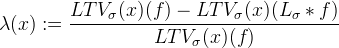
being L_σ a low pass filter. As LTV decreases very fast under low pass filtering, λ(x) gives us the local oscillatory behavior of the function.

If λ is close to 0, there is little relative reduction of the local total variation by the low pass filter. If instead λ is close to 1 the reduction is strong, which means that the considered point belongs to a textured region. Thus, a fast nonlinear low pass and high pass filter pair can be computed by doing weighted averages of f and L_σ ∗ f depending on the relative reduction of LTV

where w(x) : [0, 1] → [0, 1] is a nondecreasing piecewise affine function that is constant and equal to zero near zero and constant and equal to 1 near 1.

the soft threshold function *w(s)*

In all experiments the soft threshold parameters defining w (see the figure below) have been fixed to a₁ = 0.25 and a₂ = 0.5. If λ(x) is small the function f is non-oscillatory around x and therefore the function is BV around x. Thus u(x) = f(x) is the right choice. If instead λ is large, the function f is locally oscillatory and locally replaced by L_σ ∗ f.

The choice of λ = 1/2 as underlying hard threshold is conservative: it ensures that all step edges stay on the cartoon side, but puts all fine structures on the texture side, as soon as they oscillate more than once. Since it is desirable to have a one-parameter method, λ is fixed once and for all. In that way the method keeps the scale of the texture as the only method parameter.

Implementation

As indicated in the algorithm, the cartoon+texture decomposition only requires the application on the gradient image of two low-pass filters, which are performed directly by a discrete convolution. The gradient is computed by the simplest centered difference scheme. The main steps are:

1. Apply a low pass filter to the initial image f.

   The low pass filtered image L_σ ∗ f is obtained by convolving f with the low pass filter L_σ = (Id - (Id - G_σ)n), indicating n that the convolution is iterated n times and being n fixed to 5. Convolutions are computed in space with mirror boundary conditions, that is, the image is symmetrized out of its domain. In the current implementation this low pass filtered image is obtained iterativelly,

    low <- G_σ ∗ f 
    high <- f - low 
    for i=1:n 
        high <- high  -  G_σ ∗ high 
    low <- f - high 
   

We preferred this low pass filter to a Fourier based filter as proposed in [3], for simplicity in the coding. Next figure illustrates the low pass-high pass behavior of the proposed filter L_σ and the corresponding H_σ = Id - L_σ for several values of n.

1. Compute the Euclidian norm of the image gradients of f and L_σ ∗ f.

   The vertical and horizontal derivatives are computed by a centered two point scheme and the modulus of the gradient with an Euclidean norm.

    ux (i,j) = u(i+1,j) - u(i-1,j) 
    uy (i,j) = u(i,j+1) - u(i,j-1)
    |∇ u| = sqrt(ux(i,j)²   +  uy (i,j)²  ) 
   

2. Convolve these moduli with the Gaussian G_σ to get the local total variation of f and L_σ ∗ f.

   Convolutions are computed in space with mirror boundary conditions.

3. Deduce the value of λ(x) at each point in the image.

4. Deduce the value of the cartoon image as a weighted average of f and L_σ ∗ f.

5. Compute the texture as the difference u-f.

The color implementation for a color image f=(r,g,b) is as follows:

1. Apply a low pass filter independently to each channel of the image f.

2. Compute the local total variation of each channel of the original and low pass filtered images. Compute the color local total variation as the average of the red, green and blue local total variations.

3. Deduce the value of λ(x) at each point in the image by using the color local total variation. That is, the same function λ(x) is used for the three channels.

4. Deduce the value of the cartoon image as a weighted average of each channel of f and L_σ ∗ f.

5. Compute the texture as the difference u-f.

Examples

Cactus

The examples below illustrate several aspects of the decomposition. On the cactus image, which is large, a scale 5 is just enough to remove some detail. The borders of the cactus leaves are in no way step edges. In fact for many of them the color oscillates strongly near the edges, and is considered as texture.

sample	cartoon	texture
cactus	cartoon, scale=5	texture

Noisy Square

The second image, a noisy square on noisy background, is correctly divided into a smooth cartoon with sharp boundary and a noise texture. Notice an undesirable adhesion effect: points near the edges are considered edge points, and therefore their texture is kept in the cartoon part. This adhesion effect is observable in all images and would only be disappear if the isotropic filters were replaced by anisotropic filters.

sample	cartoon	texture
noisy square	cartoon scale=3, adhesion problem near edge	texture

Dolphin

This photograph of a logo on a boat is an almost perfect cartoon! The algorithm does well in keeping it almost entirely in the cartoon part.

sample	cartoon	texture
Dolphin: almost a cartoon	cartoon scale=4, almost identical	texture

Fingerprint

In this fingerprint image, the cartoon part only contains, as expected, a step function indicating the location of the fingerprint.

sample	cartoon	texture
fingerprint	cartoon scale=2.5	texture: almost everything

Textured Square

In this image, everything is texture. So the cartoon only contains a smoothed version of the original, and all details move on the textured part.

sample	cartoon	texture
texture square	cartoon scale =3, blurred	texture: almost everything

Other examples

sample	cartoon	texture
church door	cartoon scale=5	texture
ultrasound image	cartoon scale=5	texture
waves	cartoon scale=4	texture

Image credits

image credits