• article

@article{ipol.2011.dalmm_ps,
    title   = {{Farman Institute 3D Point Sets - High Precision 3D Data Sets}},
    author  = {Digne, Julie and Audfray, Nicolas and Lartigue, Claire and Mehdi-Souzani, Charyar and Morel, Jean-Michel},
    journal = {{Image Processing On Line}},
    volume  = {1},
    year    = {2011},
    doi     = {10.5201/ipol.2011.dalmm_ps},
}
% if your bibliography style doesn't support doi fields:
    note    = {\url{https://doi.org/10.5201/ipol.2011.dalmm_ps}}

Communicated by Jose-Luis Lisani

• Julie Digne julie.digne@cmla.ens-cachan.fr CMLA, ENS Cachan
• Nicolas Audfray nicolas.audfray@lurpa.ens-cachan.fr LURPA, ENS Cachan
• Claire Lartigue claire.lartigue@lurpa.ens-cachan.fr LURPA, ENS Cachan
• Charyar Mehdi-Souzani charyar.mehdi-souzani@lurpa.ens-cachan.fr LURPA, ENS Cachan
• Jean-Michel Morel jean-michel.morel@cmla.ens-cachan.fr CMLA, ENS Cachan

Overview

This webpage is dedicated to a new type of data: high precision raw data coming from the acquisition of objects by a 3D laser scanner.

References

1. Scale Space Meshing of Raw Data Point Sets, Digne J., Morel J.-M., Mehdi-Souzani C., Lartigue, C., Computer Graphics Forum, 2011, DOI: 10.1111/j.1467-8659.2011.01848.x
2. High Fidelity Scan Merging, Digne J., Morel J.-M., Audfray N., Lartigue, C., Computer Graphics Forum 29, no 5, pp 1643-1651, 2010, DOI: 10.1111/j.1467-8659.2010.01773.x
3. Feature extraction from high-density point clouds: toward automation of an intelligent 3D contact less digitizing strategy, Mehdi-Souzani C., Digne J. , Audfray N., Lartigue C., Morel J.-M., CAD'10, Dubai June (21-25) DOI: 10.3722/cadaps.2010.863-874
4. Scan planning strategy for a general digitized surface, Mehdi-Souzani C., Thiebaut F., Lartigue C., Journal of Computing & Information Science in Engineering, ASME International, Vol. 6, Issue 4, pp. 331-339, December 2006.DOI: 10.1115/1.2353853
5. Contact less laser-plane sensor assessment: toward a quality measurement, Mehdi-Souzani C., Lartigue C., Proceedings of IDMME-Virtual Concept 2008, Beijing, China, octobre 8-10, 2008

Acquisition process

Description

The experimental scanning device is made of three distinct parts: a displacement system, a digitizing sensor and a data processing system.

The displacement system is a Coordinate Measuring Machine (CMM) headed with a contact-free laser-plane sensor (the digitizing system). This scanner is connected to the CMM through a motorized indexing head as shown in figure 1. The two scanner head orientations are given by two angles A and B that can only be incremented by 7.5°.

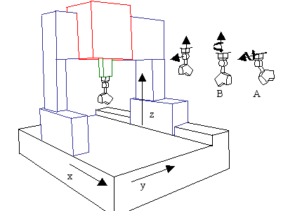
Scheme of the Acquisition System

Laser ray projected on the surface of the object to digitize

The acquisition system is based on the geometric principle of triangulation. A laser source emits a laser ray diffracted to a laser plane, and a CCD camera captures the intersection line between the laser plane and the surface of the object [4]. Since the angle between the camera and the laser ray emitter is fixed, the position of the acquired laser ray in the CCD matrix yields the 3D coordinates in the sensor coordinate system. As the position and the orientation of the scanner is known in the CMM frame, by using the calibration model of the whole system, the coordinates can be expressed in the CMM coordinate system.

Acquisition

The digital acquisition of an object needs generally several different sensor orientations. In order for a point to be acquired, it must be hit by the laser ray and seen by the CCD camera at the same time. The three translations of the CMM and the two rotations of the head allow for the high quality acquisition of freeform shapes, without repositioning the object. For each orientation, the sensor has to be calibrated on a reference measurement artefact, in this case a perfect sphere. The diameter and the position of the sphere are known with an uncertainty inferior to 0.001 mm. The center of this sphere is the origin of the CMM coordinate system. The calibration operation consists in scanning the sphere in different areas of the CCD camera [5]. As we perfectly know the size and the location of the sphere, all calibration parameters are computed for each sensor orientation. This calibration step reduces errors due to optical measurement parts of the scanner, and allows for the definition of all the objects directly in the same coordinate system. However, no digitization system is perfect. Some calibration and registration errors remain after calibration. It is nevertheless still possible to increase the quality of digitized point clouds. The distance between the captor and the object, the acquisition angle and the sensor reorientation are crucial to generate a high quality point cloud. In [5], it is shown how the error varies with respect to these settings. The result is also very dependent on the physical nature of the surface (reflectance, specularity). For some reflecting objects, a white powder has to be spread on the surface before the digitization (see the mire dataset for example).

A single sweep using a given sensor orientation is hardly enough to cover the whole surface of the object. This is due to the width of the laser ray, each sweep covers a band of the surface. Therefore, one has to do several sweeps with the same orientation only modifying the trajectory of the sensor so that it covers the whole surface.

Equipment details

We use as captor a Zephyr KZ25 manufactured by Kreon technologies. Both frequency and power of the laser ray can be set depending on the surface to probe. A Look Up Table allows for setting an intensity threshold above which a trace appearing on the CCD camera should be taken into account. The settings aim at ensuring a trace width between 7 and 9 micrometers: the laser power is set to 4mV and the integration time is 1/250s.

This captor is controlled by a rotating head. This rotating head is a Renishaw PH10M with a repeatability of 0.38 micrometers (constructor value).

The sphere used for calibration is manufactured and certified by Kreon Technologies. During the calibration stage, the difference between the computed diameter and the theoretical diameter (15,993mm) is used as well as deviation of the points relatively to a perfect sphere.

3D data file format

Each data set is given as a set of compressed ASCII files (tgz). Each file represents a single sweep in a given scanning orientation. When more than one file is provided for a single orientation, each of the corresponding files is given a number. Each file is named Ax-By_n.asc where x is the first orientation angle, y is the second orientation angle and n is the number of the sweep. The data sets are raw data point sets, in the sense that no preprocessing was applied, it is the direct output of the acquisition system.

For example, consider the "Dame de Brassempouy" dataset. It consists of 18 files:
A45_B0.asc, A45_B0_2.asc, A45_B0_3.asc, A45_B-22,5.asc, A45_B-22,5_2.asc, A90_B-180.asc, A90_B-180_2.asc, A90_B-180_3.asc, A90_B-90_2.asc, A90_B-90_3.asc, A90_B-90_4.asc, A90_B90.asc, A90_B90_2.asc, A90_B90_3.asc, A90_B90_4.asc, A90_B-135.asc, A90_B-135_2.asc, A90_B-135_3.asc

The object was acquired using 6 different orientations that can be read in the names of the files: (45,0), (45,-22.5), (90,-180), (90,-90), (90,90), (90,-135). 18 sweeps were required (corresponding to the 18 files).

Each file contains N lines (one line per points) with the point coordinates in a single row. Notice that there is no normal information.

For example, we list the 10 first lines of file A45_B0.asc, still in the "Dame de Brassempouy" dataset:

-524.21393 4.72374 -31.67768
-524.22937 4.72252 -31.76848
-524.22412 4.72135 -31.83910
-524.18768 4.72026 -31.87937
-524.16681 4.71914 -31.93484
-524.13818 4.71803 -31.98271
-524.09912 4.71696 -32.02045
-524.07050 4.71585 -32.06833
-524.04181 4.71475 -32.11621
-523.98969 4.71253 -32.21708

Each row corresponds to the x,y,z coordinates of a point of the first sweep with orientation (45,0). Coordinates are given in millimeters. The whole system is calibrated so that all coordinates are given in the same coordinate system.

A set of pictures of the data sets is also provided in a downloadable tar.gz archive. The physical size of each object (height x width x depth with respect to the provided picture), the number of sweeps and the total point number are also given.

Data

The objects presented here are reproductions bought from Le Louvre Museum, Paris, France (http://www.boutiquesdemusees.fr/en/), with the exception of the mask and tanagra which come from the Museum of Cycladic Arts (Athens, Greece). Most of the objects are made of resin.

Tanagra

data set
high-resolution photographs
object size: 22 × 7.5 × 9 cm
(160 sweeps, 17,496,999 points, 186MBytes)

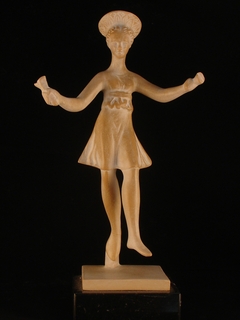
Dancer with Crotales

data set
high-resolution photographs
object size: 20 × 11 × 6 cm
(94 sweeps, 5,524,627 points, 60MBytes)

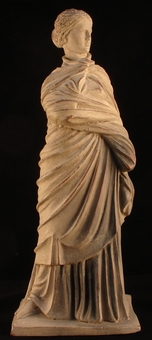
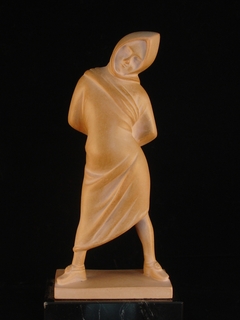
Mime

data set
high-resolution photographs
object size: 17.5 × 7 × 5 cm
(102 sweeps, 8,611,522 points, 93MBytes)

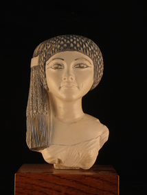
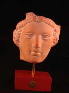
Nefertiti

data set
high-resolution photographs
object size: 19 × 11 × 6 cm
(115 sweeps, 15,554,528 points, 168MBytes)

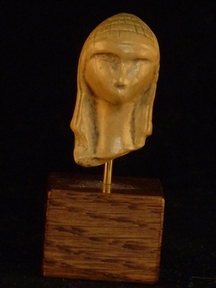
Dame de Brassempouy

data set
high-resolution photographs
object size: 6 × 2 × 2 cm
(18 sweeps, 319,220 points, 3.5MBytes)

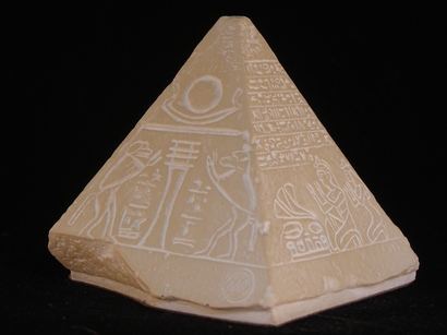
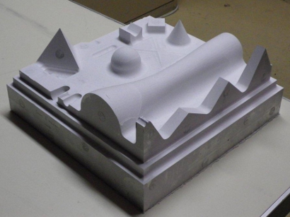
Pyramid

data set
high-resolution photographs
object size: 8 × 7.5 × 7.5 cm
(41 sweeps, 5,632,884 points, 59MBytes)

Mask

data set
high-resolution photographs
object size: 16 × 10 × 6 cm
(78 sweeps, 8,961,736 points, 99MBytes)

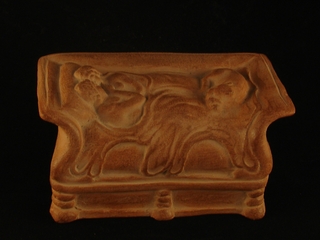
Amants de Bordeaux

data set
high-resolution photographs
object size: 8 × 13 x 7 cm
(70 sweeps, 15,835,405 points, 168MBytes)

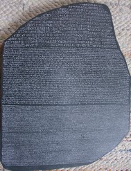
Rosetta Stone

data set
high-resolution photographs
object size: 32 × 25.5 × 1.5 cm
(62 sweeps, 36,201,537 points, 363MBytes)

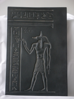
Anubis Bas-relief

data set
high-resolution photographs
object size: 30 × 20 × 2 cm
(13 sweeps, 9,991,040 points, 97MBytes)

Mire

data set
high-resolution photographs Object size: 7 x 15 × 15 cm (75 sweeps, 16,111,522 points, 173MBytes)

Reading the data

The files are in plain ASCII. Reading them is straightforward from C or C++ (or any other programming language). We provide an example of a C++ program that reads points from a file "example.txt" and outputs all the points (one point per line) on the standard output.

#include<iostream>
#include<fstream>


using namespace std;

/**reads and display the content of a file
 * */
int main()
{
//stream to read the file
ifstream in;

//opening the file
in.open("example.txt");

//variables to get the coordinates of the point
double x,y,z;

//reading the data from the file
in>>x>>y>>z;

while(!in.eof())//read in the file while not at the end of the file
{
    //displaying the data, one point per line (this part should be replaced by whatever you want to do with the data)
    cout<<x<<"\t"<<y<<"\t"<<z<<endl;

    //reading the data from the file
    in>>x>>y>>z;

}
//closing the file
in.close();
return EXIT_SUCCESS;
}

Visualizing the data

Visualization of unoriented and non triangulated 3D point clouds is a difficult problem. In this case the clouds are so dense that it would result in visualizing the silhouette of the shape. However, if for some reason, the point cloud has to be visualized then the following MATLAB/Octave routine is sufficient:

A=load('data.txt');
plot3(A(:,1),A(:,2),A(:,3),'.');axis equal;