@article{ipol.2011.g_lmii,
    title   = {{Linear Methods for Image Interpolation}},
    author  = {Getreuer, Pascal},
    journal = {{Image Processing On Line}},
    volume  = {1},
    year    = {2011},
    doi     = {10.5201/ipol.2011.g_lmii},
}
% if your bibliography style doesn't support doi fields:
    note    = {\url{http://dx.doi.org/10.5201/ipol.2011.g_lmii}}
- published
- 2011-09-27
- reference
- Pascal Getreuer, Linear Methods for Image Interpolation, Image Processing On Line, 1 (2011). http://dx.doi.org/10.5201/ipol.2011.g_lmii
Communicated by Gabriele Facciolo
Demo edited by Pascal Getreuer
- Pascal Getreuer
pascal.getreuer@cmla.ens-cachan.fr, CMLA, ENS Cachan
Overview
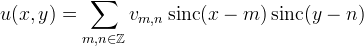
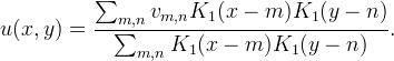
Given input image v with uniformly-sampled pixels vm,n, the goal of interpolation is to find a function u(x,y) satisfying

such that u approximates the underlying function from which v was sampled. Another way to interpret this is v was created by subsampling, and interpolation attempts to invert this process.
We discuss linear methods for interpolation, including nearest neighbor, bilinear, bicubic, splines, and sinc interpolation. We focus on separable interpolation, so most of what is said applies to one-dimensional interpolation as well as N-dimensional separable interpolation.
References
- C.E. Shannon, “A Mathematical Theory of Communication,“ Bell System Technical Journal, vol. 27, pp. 379–423, 623–656, 1948.
- G. Strang and G. Fix, “A Fourier analysis of the finite element variational method,” Constructive Aspects of Functional Analysis, Edizioni Cremonese, Rome, pp. 795–840, 1973.
- R. Keys, “Cubic Convolution Interpolation for Digital Image Processing,” IEEE Trans. Acoustics, Speech, and Signal Processing, 29(6), 1981.
- A. Aldroubi, M. Unser, and M. Eden, “Cardinal spline filters: stability and convergence to the ideal sinc interpolator,” Signal Processing, vol. 28, no. 2, pp. 127–138, 1992.
- A. Schaum, “Theory and design of local interpolators,” CVGIP: Graph. Models Image Processing, vol. 55, no. 6, pp. 464–481, 1993.
- M. Unser, “Splines: A Perfect Fit for Signal/Image Processing,” IEEE Signal Processing Magazine, 16(6), pp. 22–38, 1999.
- P. Thévenaz, T. Blu, and M. Unser, “Interpolation Revisited,” IEEE Trans. Medical Imaging, vol. 19, no. 7, pp. 739–758, 2000.
- T. Blu, P. Thévenaz, and M. Unser, “MOMS: Maximal-Order Interpolation of Minimal Support,” IEEE Trans. Image Processing, vol. 10, no. 7, pp. 1069–1080, 2001.
- E. Meijering, “A Chronology of Interpolation: From Ancient Astronomy to Modern Signal and Image Processing,” In Proceedings of the IEEE, 90, pp. 319–342, 2002.
- F. Malgouyres and F. Guichard, “Edge direction preserving image zooming: A mathematical and numerical analysis,” SIAM J. Numerical Analysis, 39(1), pp. 1–37, 2002.
- B. Fornberg, E. Larsson, N. Flyer, “Stable computations with Gaussian radial basis functions,” SIAM J. Sci. Comput. 33, pp. 869–892, 2011.
- FFmpeg, http://www.ffmpeg.org.
Online Demo
An online demo of this algorithm is available.
Notations
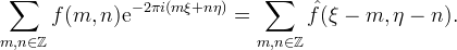
We use the following normalization of the Fourier transform,
the transform of a function f is denoted by hat. We will also use the bilateral Z-transform. The Z-transform of a sequence cn is
We denote the sequence with a subscript cn and its Z-transform as c(z).
Interpolation Kernels
Linear interpolation can be abstractly described as a linear operator Z mapping samples v to a function u := Z(v). We define two properties on Z.
Let Sk,l denote shifting, Sk,l(v)(m,n) := vm−k,n−l. Z is said to be shift-invariant if for every v and (k, l),

Let vN denote the restriction of v to the set {−N,…,+N}2, then Z is said to be local if for every v and (x, y),
If Z is a linear, shift-invariant, local operator from  to
to  , then there exists a unique function K ∈ L1 called the interpolation kernel such that Z(v) can be written as a convolution [10]:
The conditions for this result are mild and are satisfied by most linear interpolation methods of practical interest.
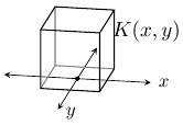
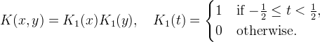
The properties of the kernel K, like symmetry, regularity, and moments, imply properties of the interpolation. For four-fold rotational symmetry, K is usually designed as a tensor product K(x,y) = K1(x)K1(y), where K1 is a symmetric function. Such a kernel also has the benefit that the interpolation is separable, the interpolation can be decomposed into one-dimensional interpolations along each dimension.
Similarly in three (or higher) dimensions, it is convenient to use a separable kernel K(x,y,z) = K1(x)K1(y)K1(z) so that the interpolation decomposes into one-dimensional interpolations. More generally, one can use different one-dimensional kernels along different dimensions, K(x,y,z) = K1(x)K2(y)K3(z). For instance, it may be more appropriate to use a different kernel for the temporal dimension than for the spatial dimensions in video interpolation.
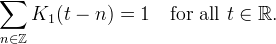
In order to have the interpolant agree with the known samples Z(v)(m,n) = vm,n, it is easy to see that the requirements are K(m,n) = 0 for all integer m and n, except at the origin where K(0,0) = 1. K is said to be an interpolating function if it satisfies these requirements.
Two-Step Interpolation
That K must be interpolating can be an inconvenient restriction. It complicates the problem of finding a kernel K that also satisfies other design objectives. It can also be an obstacle computationally. In some cases such as spline interpolation, K has infinite support, yet the interpolant can be expressed as a linear combination of compact support functions (the B-splines).
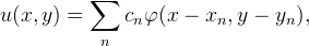
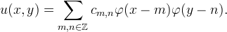
Suppose that one dimensional data fm is to be interpolated. An alternative approach is to begin with a basis function φ(t) and then express the interpolant as a linear combination of {φ(t − n)},
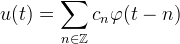
where the coefficients cn are selected such that
That is, interpolation is a two-step procedure: first, we solve for the coefficients cn and second, the interpolant is constructed as ∑cnφ(t − n).
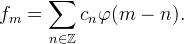
To solve for the coefficients, notice that fm = ∑cnφ(m − n) is equivalent to a discrete convolution fm = (c ∗ p)m where pm = φ(m). This suggests solving for cn under the Z-transform as
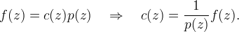
Let (p)−1 deonte the convolution inverse of p, which is the sequence such that p ∗ (p)−1 = δ where δ is the unit impulse (δ0 := 1 and δm := 0 otherwise). Using (p)−1 we obtain cn by “prefiltering” as
A unique convolution inverse exists in many practical cases of interest [7]. If it exists and φ is real and symmetric, then (p)−1 can be factored into pairs of recursive (infinite impulse response) filters, allowing for an efficient in-place calculation. Finally, the interpolant is obtained as ∑cnφ(t − n).
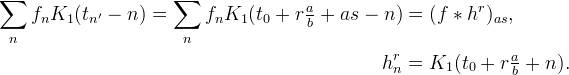
It is possible to express this two-step interpolation procedure in terms of an interpolation kernel,
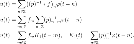
For example, the following figures illustrate this relationship for cubic and septic (7th) B-spline interpolation where φ are the cubic and septic B-splines. In both cases, φ is not an interpolating function, but prefiltering with (p)−1 yields a kernel K1 that is interpolating.
 |
| Two-step interpolation where φ is the cubic B-spline. |
 |
| Two-step interpolation where φ is the septic B-spline. |
Interpolation Properties
An interpolation method Z has approximation order J if it reproduces polynomials up to degree (J − 1).
Let Z and K1 be defined from a function φ as in the previous section. The Strang–Fix conditions [2] provide the following equivalent conditions to determine the approximation order.
- Z has approximation order J,


where  denotes the j_th derivative of
  and
and  . Aside from approximation order, another property of interest is the L2 interpolation error. Let
  and define fδ(t) = ∑f(δn)K1(t − n) for δ_ > 0. The interpolation error is approximately
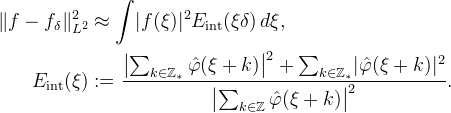
This approximation is exact for bandlimited functions. Otherwise, it is equal to the average L2 error over all translations of f. The function Eint is called the interpolation error kernel, and it can be interpreted as predicting the error made in interpolating sin(2πξt). Asymptotically as δ → 0,
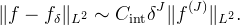
The decay of the error is dominated by the approximation order J. When comparing methods of the same approximation order, the constant Cint is also of interest [7].
Kernel Normalization
A basic and desirable quality of an interpolation method is that it reproduces constants, which is equivalent to
If the kernel does not reproduce constants, it can be the normalized to fix this as
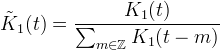
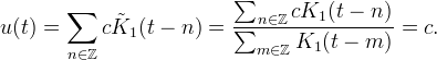
provided that the denominator does not vanish. Normalization ensures that the interpolation weights sum to 1. Interpolation with the normalized kernel reproduces constants: suppose fn = c, then
Nearest Neighbor
The most widely used methods for image interpolation are nearest neighbor, bilinear, and bicubic interpolation.
| Nearest Neighbor | Bilinear | Bicubic |
 |
 |
 |
| Nearest neighbor, bilinear, and bicubic applied to the same uniformly-spaced input data. | ||
The nearest neighbor interpolation of v is the piecewise constant function
![u(x,y) = v_{[x],[y]}](./g_lmii/dd964fd961271863f715f547e1352395.png)
where [⋅] denotes rounding to the nearest integer. That is, u(x,y) is defined as the value of the input sample that is closest to (x,y). For this reason, nearest neighbor interpolation is sometimes called “pixel duplication.” The interpolation kernel for nearest neighbor is
The nearest neighbor idea can be applied to very general kinds of data, to any set of samples that has a notion of distance between sample locations. The interpolant is constant within the Voronoi cell around each sample location.
 |
| Nearest neighbor scattered data interpolation. |
Bilinear
The bilinear interpolation of v is the continuous function

where ⌊⋅⌋ denotes the floor function and 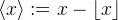 is the fractional part. The interpolation kernel is

where (⋅)+ denotes positive part.
Within each cell [m,m+1]×[n,n+1], the interpolation is a convex combination of the samples located at the cell corners vm,n, vm+1,n, vm,n+1, vm+1,n+1. Because this combination is convex, the interpolation is bounded between min v and max v and does not produce overshoot artifacts. Bilinear interpolation reproduces affine functions: if vm,n = am + bn + c then u(x,y) = ax + by + c.
Bilinear interpolation is arguably the simplest possible separable method that produces a continuous function. It is extremely efficient and on many platforms available in hardware, making it practical for realtime applications.
A closely related method to bilinear interpolation is linear interpolation. Given a triangulation of the sample locations, each triangle is interpolated by the affine function that satisfies the data at the triangle vertices.
Bicubic
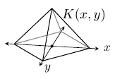
 |
| Cubic interpolation kernel. |
 |
| Surface plot of K1(x)K1(y). Yellow circles indicate local maxima. |
Bicubic interpolation [3] uses the interpolation kernel
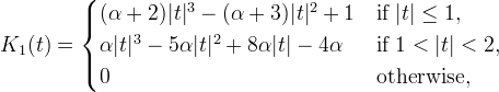
where α is a free parameter. This function is derived by finding a piecewise cubic polynomial with knots at the integers that is required to be symmetric, C1 continuous, and have support in −2<t<2. These conditions leave one remaining degree of freedom represented by α. For any value of α, K1 has extremal points at t = 0 and ±4/3.
The values −1, −0.75, and −0.5 have been proposed for α, motivated by various notions of optimality [9]. The choice α = −0.5 is particularly compelling. Bicubic interpolation is third-order accurate with α = −0.5 and only first-order accurate for any other α. Furthermore, α = −0.5 is optimal in a sense of matching the sinc kernel and is also optimal in terms of Eint. All examples and comparisons with bicubic here use α = −0.5.
 |
| Comparison of the nearest neighbor, bilinear, and bicubic kernels and the sinc. |
Sinc
 |
| The sinc function. |
 |
| Surface plot of sinc(x)sinc(y). Yellow circles indicate local maxima. |
The Whittaker–Shannon interpolation [1] of v is
where sinc(t) := sin(πt)/(πt) for t ≠ 0 and sinc(0) := 1 is the interpolation kernel. The interpolation is such that u is bandlimited, that is, its Fourier transform is zero for frequencies outside of [−½,½]. This interpolation is also often called “sinc interpolation” or “Fourier zero-padding.” The extremal points of the sinc kernel are solutions of the equation πt = tan(πt), which include t ≈ 0, ±1.4303, ±2.4590, ±3.4709, ±4.4774.
The powerful property of sinc interpolation is that it is exact for bandlimited functions, that is, if vm,n = f(m,n) with

then the interpolation reproduces f. Proof

 if
if  is zero outside of the region
 In some ways, sinc interpolation is the ultimate interpolation. It is exact for bandlimited functions, so the method is very accurate on smooth data. Additionally, Fourier zero-padding avoids staircase artifacts, it is effective in reconstructing features at different orientations. Under an aliasing condition [10], Fourier interpolation reproduces cylindrical functions f(x,y) = h(αx + βy).
The disadvantage of sinc interpolation is that in aliased images it produces significant ripple artifacts (Gibbs phenomenon) in the vicinity of image edges. This is because sinc(x) decays slowly, at a rate of 1/x, so the damage from meeting an edge is spread throughout the image. Moreover, bandlimitedness can be a distorted view of reality. Thévenaz et al. [7] give the following amusing example: consider the air/matter interface of a patient in a CT scan, then according to classical physics, this is an abrupt discontinuity and cannot be expressed as a bandlimited function. Antialias filtering is not possible on physical matter, and any attempt to do so would probably be harmful to the patient.
| Nearest Neighbor | Bilinear | Bicubic | Lanczos-3 | Cubic B-Spline | Sinc |
 |
 |
 |
 |
 |
 |
| Linear interpolation of a step edge: a balance between staircase artifacts and ripples. | |||||
Windowed Sinc Approximations
 |
| The Lanczos-3 kernel. |
 |
| Surface plot of the Lanczos-3 kernel. Yellow circles indicate local maxima. |
A solution to limiting the ripple artifacts of the sinc kernel is to approximate it with a compactly-supported function
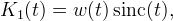
where w is a window function. A popular choice in image processing is the Lanczos window,
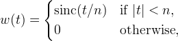
where n is a positive integer usually set to 2 or 3. The Lanczos kernels do not reproduce constants exactly, but can be normalized to fix this as described in the section on Kernel Normalization. There are many other possibilities for the window, for example Hamming, Kaiser, and Dolph–Chebyshev windows to name a few, each making different tradeoffs in frequency characteristics.
 |
| Comparison of the normalized Lanczos kernels and the sinc. |
The cubic B-spline.
Splines
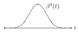
Define the B-splines,
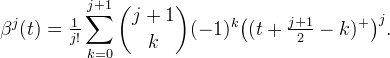
The B-spline functions are optimal in the sense that, among all piecewise polynomials with uniformly spaced knots, the B-splines have the maximal approximation order and are maximally continuous for a given support.
The B-spline βJ−1 has approximation order J. For J > 2, βJ−1 is not interpolating, so prefilting must be applied as described in the section on Two-Step Interpolation where βJ−1 takes the role of φ.
As J→∞, B-spline interpolation converges to Whittaker–Shannon interpolation in a strong sense: the associated interpolation kernel K1 converges to the sinc both in the spatial and Fourier domains in Lp for any 1 ≤ p < ∞, see [4], [6]. This convergence is illustrated in the figure below with K1 and its Fourier transform for degrees 1, 3, 5, and 7.
 |
| Comparison of the B-spline interpolation kernels and the sinc. |
Aside from the B-splines, there are numerous other piecewise polynomial methods for interpolation in the literature. One example is the class of Maximum Order and Minimal Support (Moms) functions introduced by Blu, Thévenaz, and Unser [8], which are linear combinations of βJ−1 and its derivatives,
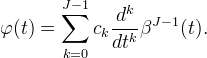
The B-splines are a special case within the class of Moms. The B-splines are the Moms with maximum regularity, they are (J − 2) times continuously differentiable.
Within the Moms, the “o-Moms functions” are the Moms defined by minimizing the quantity
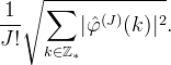
The o-Moms functions have the same approximation order and support as the B-splines, but the Cint constant is smaller. So compared to the B-splines, the advantage of o-Moms is that they have lower asymptotic L2 interpolation error. On the other hand, o-Moms are less regular than the B-splines.
The splines proposed by Schaum [5] are also within the class of Moms. Schaum splines have the property that they are interpolating, so prefiltering is not needed. However, for a given support size, the approximation constant Cint is worse than with the o-Moms of the same support.
The first few even-order o-Moms are
| Order J | φ(t) | |
| 2 |  | |
| 4 | 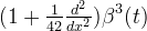 | |
| 6 | 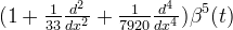 | |
| 8 |  | |
| 10 |  | |
| 12 |  |
A note on numbering: Usually, with a piecewise polynomial method, its approximation order is L but its highest degree is (L − 1). We refer to methods by degree, for instance “o-Moms 3” and “β3” are methods that are locally cubic polynomial and have approximation order 4.
Radial Basis Functions
A radial basis function (RBF) is a function φ such that

RBF interpolation is useful for scattered data interpolation. Let (xn,yn) denote the location of the nth sample, then the interpolant is
where the coefficients cn are solved such that u(xn,yn) = vn. If the samples are uniformly spaced, then the cn can be found as described in the section on Two-Step Interpolation.
Popular choices for φ include
| • | Thin plate splines | φ(r) = |εr|nlog|εr|, n even |
| • | Bessel | φ(r) = J0(εr) |
| • | Gaussian | φ(r) = exp(−(εr)2) |
| • | Multiquadric | φ(r) = (1 + (εr)2)½ |
| • | Inverse multiquadric | φ(r) = (1 + (εr)2)−½ |
| • | Inverse quadratic | φ(r) = (1 + (εr)2)−1 |
where ε is a positive parameter controlling the shape. A challenging problem is that smaller ε improves interpolation quality but worsens the numerical conditioning of solving the cn. A topic of interest beyond the scope of this article is RBF interpolation in the limit ε → 0. For example, [11] investigates numerically stable interpolation for small ε with Gaussian φ.
Methodology
Boundary handling
A technicality is how to handle the image boundaries. The interpolation formulas may refer to samples that are outside of the domain of definition, especially when interpolating at points near or on the image boundaries.
The usual approach is to extrapolate (pad) the input image. Several methods for doing this are
- Constant extension, …aaaabcdeeee…
- Half-sample symmetric extension, …cbaabcdeedc…
- Whole-sample symmetric extension, …dcbabcdedcb…
Image scaling
Suppose v is an M×N image with samples vm,n, m = 0,…M − 1, n = 0,…N − 1, which are located on the integer grid  .
.
For scaling v by a (possibly non-integer) factor d, a choice for where to resample the function u is on a top-left-anchored grid of points

with M ′ = [dM], N ′ = [dN], where [⋅] is a rounding convention.
 |
| Example top-left-anchored grids. Open circles denote input samples and filled circles denote interpolation samples. |
Another choice is the centered grid of points

where sr,M,M ′ = (1/d − 1 + M − M ′ /d)/2. If d is integer, the offsets simplify to s = (1/d − 1)/2. Although more complicated, the centered grid has the advantage that interpolation with a symmetric kernel on this grid commutes with flipping the image.
 |
| Example centered grids. Open circles denote input samples and filled circles denote interpolation samples. |
For an odd integer scale factor and interpolation with a symmetric kernel, the two grids are related in a simple way through adding and removing border samples. Interpolation performed on the top-left-anchored grid is converted to an interpolation on the centered grid by removing (d − 1)/2 rows and columns from the bottom and right borders and extrapolating (according to the boundary extension) the same number of rows and columns on the top and left.
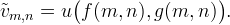
Domain mapping
Aside from changing image resolution, another application is to deform or map the domain of the image. That is, the mapped coordinates (x',y') are related to the original coordinates (x,y) by

Let u(x,y) be an interpolation of v, then the deformed image is obtained by resampling as
For example, two simple mappings are
- Sub-pixel translation
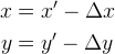
- Rotation
Other applications include parallax correction, lens distortion correction, image registration, and texture mapping.
Algorithm
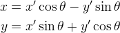
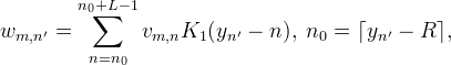
Linear interpolation amounts to evaluating the sum
Choices of algorithms to do this efficiently depend on K and the sampling locations. Keep in mind that the sum is conceptually over the infinite integer grid, so vm,n should be replaced with an appropriate boundary extension when m,n is beyond the domain of the image.
Nearest neighbor, bilinear, and bicubic
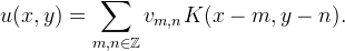
Suppose the interpolation method has a separable kernel K(x,y) = K1(x)K1(y) with compact support, K1(x) = 0 for x ≥ R. Then interpolation at point (x,y) can be implemented as
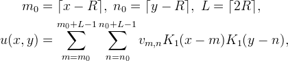
where there are L×L nonzero terms in the sum. The values of K1 can be reused so that K1 only needs to be evaluated for only 2_L_ different arguments.
For image scaling, it is possible to interpolate more efficiently by exploiting the separable structure of the sampling points. Let vm,n, m = 0,…, M − 1, n = 0,…, N − 1 be the given image, which is to be interpolated on the grid of points (xm′,yn′) for m′ = 0,…, M ′ − 1, n′ = 0,…, N ′ − 1. Interpolation is performed by first interpolating along the y direction,
for m = 0,…, M − 1, n′ = 0,…, N ′ − 1, and then along the x direction,
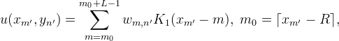
for m′ = 0,…, M ′ − 1, n′ = 0,…, N ′ − 1.
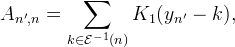
An efficient way to implement the one dimensional interpolations is to express them as multiplication with a sparse matrix:

A is a sparse matrix of size N ′ × N and B is a sparse matrix of size M ′ × M. Away from the boundaries, the matrix entries are

Near the boundaries, the matrix entries need to be adjusted according to the boundary extension. Define
| Half-sample symmetric |  |
| Whole-sample symmetric |  |
| Constant extension | 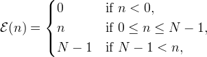 |
then the matrix entries near the boundaries are computed as
and similarly for B. This sparse matrix approach is used by the libswscale library in FFmpeg [12] for scaling video frames. It is especially well-suited for video, as A and B only need to be constructed once to interpolate any number of frames.
If the interpolation locations are uniformly spaced with a rational period, tn′ = t0 + n′⋅a/b, then another approach is to compute one-dimensional interpolation through convolution. Given n′, let s = b⌊n′/b⌋ and r be such that n′ = bs + r, then
Lanczos
Interpolation with the Lanczos kernels does not exactly reproduce constants. To fix this, the Lanczos kernels should be normalized as described in the section on Kernel Normalization.
Kernel normalization can be incorporated efficiently into the algorithms discussed in the previous section. For the interpolation of a single point (x,y), the normalized interpolation is
For the sparse matrix approach, kernel normalization is achieved by scaling each matrix row so that it sums to one. Similarly for the convolution approach, hr should be scaled so that it sums to one.
Splines
For spline methods, implementation is as described in the section on Two-Step Interpolation. The method is determined by the choice of basis function φ, for example, φ may be a B-spline or an o-Moms function.
Given a basis function φ, define pm = φ(m). For the prefiltering step, the convolution inverse (p)−1 is needed. We look first at the cubic B-spline as an example. For the cubic B-spline, p(z) = (z + 4 + z−1)/6 and
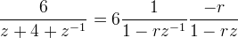
where r = 3½ − 2. The first factor corresponds to the first-order causal recursive filter

The left endpoint c'0 can be computed depending on the boundary extension,
| Half-sample symmetric | 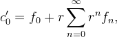 |
| Whole-sample symmetric | 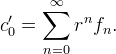 |
Since |r| < 1, the terms of the sum are decaying, so in practice we only evaluate as many terms as are needed for the desired accuracy.
The second factor corresponds to the first-order anti-causal recursive filter

The right endpoint c''N−1 can be computed according to the boundary extension as
| Half-sample symmetric | 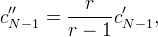 |
| Whole-sample symmetric | 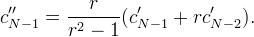 |
Finally, the constant scale factor is applied cn = 6_c''n_. The cost of prefiltering is linear in the number of pixels. Prefiltering can be computed in-place so that the prefiltered values overwrite the memory used by the input. For prefiltering in two-dimensions, the image is first prefiltered along each column, then the column-prefiltered image is prefiltered along each row.
More generally, if φ is symmetric and compactly supported, then p(z) has the form
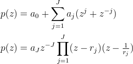
where the rj and 1/rj are the roots of the polynomial z−Jp(z). We enumerate the roots so that |rj| < 1. The Z-transform of (p)−1 is
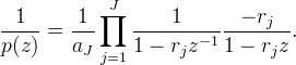
Therefore, prefiltering can be performed as a cascade of first-order recursive filters using the same algorithm as for the cubic B-spline. The table below lists the roots and the constant scale factor for several B-splines and o-Moms.
|
|
Once the image has been prefiltered c = (p)−1 ∗ v, interpolation at a point (x,y) is computed as
This second step is essentially the same formula as in the section on nearest neighbor, bilinear, and bicubic, and the same algorithms can be used to perform this step. The only differences are that the prefiltered image c is used in place of v and φ is used in place of K1.
Sinc
For sinc interpolation with an integer scale factor, interpolation can be implemented using the fast Fourier transform (FFT). This approach follows from observing that the sinc interpolant is the unique image that is bandlimited and agrees with the input data.
The input image is first padded to twice its size in each dimension with half-symmetric extension and transformed with the FFT. The interpolation is then constructed in the Fourier domain by copying the transform coefficients of the padded input image for the lower frequencies and filling zeros for the higher frequencies. The final interpolation is obtained by inverse FFT and removal of the symmetric padding. For real-valued input data, some computational savings can be made by using a real-to-complex FFT and complex-to-real inverse FFT to exploit the complex conjugate redundancy in the transform. The complexity of the interpolation is O(N log N) for N output pixels.
Implementation
This software is distributed under the terms of the simplified BSD license.
- source code zip tar.gz
- online documentation
Fourier transforms are implemented using the FFTW library.
Please see the readme.html file or the online documentation for details.
Examples
Scaling smooth data
The smooth function cos((x2 + y2)/10) is sampled on the grid {0.5,1.5,…,15.5}×{-15.5,-14.5,…,15.5} and interpolated on the centered grid with scale factor 4. The figure below compares the interpolation result using various linear methods, along with the root mean squared errors (RMSE) between the interpolation and the exact image.
| Exact | Nearest RMSE 59.2 |
Bilinear RMSE 47.2 |
Bicubic RMSE 39.0 |
Lancoz 2 RMSE 38.8 |
Lancoz 3 RMSE 33.8 |
Lanczos 4 RMSE 31.9 |
Sinc RMSE 27.2 |
 |
 |
 |
 |
 |
 |
 |
 |
| β3 RMSE 33.7 |
o-Moms 3 RMSE 31.8 |
β5 RMSE 30.9 |
o-Moms 5 RMSE 30.4 |
β7 RMSE 29.7 |
o-Moms 7 RMSE 29.4 |
β9 RMSE 29.0 |
β11 RMSE 28.5 |
 |
 |
 |
 |
 |
 |
 |
 |
For this example, higher-order methods tend to perform better. The o-Moms perform slightly better than the B-splines of the same order. Sinc interpolation yields the best result.
Scaling piecewise smooth data
We repeat the previous experiment with piecewise smooth data. The image is discontinuous at the edges, so the bandlimited hypothesis of sinc interpolation is severely violated. Sinc interpolation and other higher-order methods produce strong artifacts near edges. The bicubic and Lanczos-2 interpolations have the lowest RMSE in this case.
| Exact | Nearest RMSE 32.2 |
Bilinear RMSE 25.6 |
Bicubic RMSE 24.5 |
Lancoz 2 RMSE 24.5 |
Lancoz 3 RMSE 24.8 |
Lanczos 4 RMSE 25.1 |
Sinc RMSE 26.3 |
 |
 |
 |
 |
 |
 |
 |
 |
| β3 RMSE 24.7 |
o-Moms 3 RMSE 24.9 |
β5 RMSE 25.1 |
o-Moms 5 RMSE 25.2 |
β7 RMSE 25.4 |
o-Moms 7 RMSE 25.5 |
β9 RMSE 25.6 |
β11 RMSE 25.7 |
 |
 |
 |
 |
 |
 |
 |
 |
Texture mapping
A 3D scene of a plane and a sphere is texture mapped with an image. Texture mapping is an example of domain mapping, where in this case the image domain is mapped to the projected plane and sphere surfaces.
| Texture | Nearest | Bicubic |
 |
 |
 |
This mapping is derived through reverse ray tracing. For each pixel of the rendering of the 3D scene, a ray of light is virtually traced in reverse. The light ray begins from the eye of the observer, passes through a pixel of the screen, and continues into the 3D scene. The ray may then intersect the plane or the sphere (or nothing, if the ray continues into the background).
 |
| Reverse ray tracing. A ray of light is traced from the observer into the 3D scene. |
The ray's intersection point (X,Y,Z) with the 3D scene determines the color of its pixel. The plane is texture mapped as x = X mod M, y = Z mod N. The sphere is texture mapped as x = θ, y = φ, where θ and φ are the spherical angles of the intersection.
Image rotation
Image rotation is another application that for a general rotation angle requires interpolation. The choice of interpolation method significantly affects the quality of the output image. In this experiment, an image is successively rotated by 5 degrees increments using several linear methods. The initial image is rotated by 5 degrees, then the rotated image is rotated by another 5 degrees, and so on.
| Nearest | Bilinear | Bicubic | β11 |
 |
|||
Rotation using nearest neighbor produces jagged artifacts along edges. Rotation with bilinear is much better but blurs the image. Rotation with bicubic is sharper, but blurring is still noticeable. Finally, the sharpest rotation among these results is with the 11th order B-spline β11. By interpolating with a high-order B-spline, it closely approximates rotation via sinc interpolation.
This material is based upon work supported by the National Science Foundation under Award No. DMS-1004694. Any opinions, findings, and conclusions or recommendations expressed in this material are those of the author(s) and do not necessarily reflect the views of the National Science Foundation. Work partially supported by the MISS project of Centre National d'Etudes Spatiales, the Office of Naval Research under grant N00014-97-1-0839 and by the European Research Council, advanced grant “Twelve labours.”


