• article
• demo
• archive

@article{ipol.2011.g_mhcd,
    title   = {{Malvar-He-Cutler Linear Image Demosaicking}},
    author  = {Getreuer, Pascal},
    journal = {{Image Processing On Line}},
    volume  = {1},
    year    = {2011},
    doi     = {10.5201/ipol.2011.g_mhcd},
}
% if your bibliography style doesn't support doi fields:
    note    = {\url{http://dx.doi.org/10.5201/ipol.2011.g_mhcd}}

Communicated by Antoni Buadès
Demo edited by Pascal Getreuer

• Pascal Getreuer pascal.getreuer@cmla.ens-cachan.fr, CMLA, ENS Cachan

Overview

Image demosaicking (or demosaicing) is the interpolation problem of estimating complete color information for an image that has been captured through a color filter array (CFA), particularly on the Bayer pattern. While many complicated methods for demosaicking have been proposed, Malvar, He, and Cutler [5] showed that surprisingly good results are possible with a simple linear method using 5×5 filters.

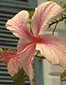
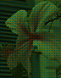
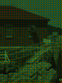
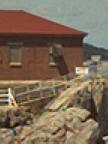
Exact	Observed Image	Demosaicked Image
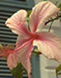Malvar, He, and Cutler's demosaicking. The images are enlarged to show individual pixels more clearly.

In the Bayer pattern [1], green pixels cover half the array in a quincunx lattice. The red and blue pixel locations are spaced uniformly every two pixels. The pattern alternates between “red rows” and “blue rows.” In a red row the pattern is R, G, R, G, …, and in a blue row it is G, B, G, B, ….

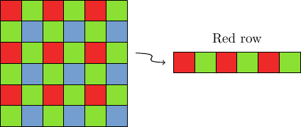The Bayer pattern.

References

1. B. E. Bayer, “Color imaging array,” U.S. Patent 3971065, 1976.
2. J. F. Hamilton, Jr. and J. E. Adams, Jr., “Adaptive color plan interpolation in single sensor color electronic camera,” U.S. Patent 5629734, 1997.
3. S.-C. Pei and I.-K. Tam, “Effective color interpolation in CCD color filter array using signal correlation,” Proc. ICIP, pp. 488–491, Sept. 2000.
4. B. K. Gunturk, Y. Altunbasak, and R. M. Mersereau, “Color plane interpolation using alternating projections,” IEEE Transactions on Image Processing, vol. 11, no. 9, pp. 997–1013, 2002.
5. Henrique S. Malvar, Li-wei He, Ross Cutler, “High-quality linear interpolation for demosaicing of Bayer-patterned color images,” in Proc. of IEEE ICASSP, 2004.
6. Xin Li, “Demosaicing by successive approximation,” IEEE Transactions on Image Processing, vol. 14, no. 3, pp. 370–379, 2005.
7. Lei Zhang and Xiaolin Wu, “Color demosaicking via directional linear minimum mean square-error estimation,” IEEE Transactions on Image Processing, vol. 14, no. 12, pp. 2167–2178, 2005.
8. Henrique S. Malvar, Li-wei He, Ross Cutler, “High-quality gradient-corrected linear interpolation for demosaicing of color images,” U.S. Patent 7502505, 2009.
9. Antoni Buades, Bartomeu Coll, Jean-Michel Morel, Catalina Sbert, “Self-Similarity Driven Demosaicking” Image Processing On Line.

Online Demo

An online demo of this algorithm is available.

Algorithm

The method is derived as a modification of bilinear interpolation. Let R, G, B denote the red, green, and blue channels. At a red or blue pixel location, the bilinear interpolation of the green component is the average of its four axial neighbors,

Bilinear interpolation of the red and blue components is similar, but using instead the four diagonal neighbors.

The visual quality of bilinear demosaicking is generally quite poor. Since the channels are interpolated independently, the misalignments near edges produce strong color distortions and zipper artifacts.

To improve upon the quality of the bilinear method, Malvar, He, and Cutler follow the work of Pei and Tam [3] by adding Laplacian cross-channel corrections. The green component at a red pixel location is estimated as

where Δ_R is the discrete 5-point Laplacian of the red channel,

To estimate a red component at a green pixel location,

where Δ_G is a discrete 9-point Laplacian of the green channel. To estimate a red component at a blue pixel location,

where Δ_B is the discrete 5-point Laplacian of the blue channel. By symmetry, blue components are estimated in a manner similar to the estimation of the red components. These formulas are shown in more detail in the next section.

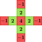
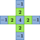
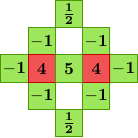
The parameters α, β, γ control the weight of the Laplacian correction terms. To set these parameters optimally, the values producing the minimum mean squared error over the Kodak image suite were computed. These values were then rounded to dyadic rationals to obtain

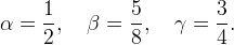
The advantage of this rounding is that the filters may be efficiently implemented with integer arithmetic and bitshifting. The filters approximate the optimal Wiener filters within 5% in terms of mean squared error for a 5×5 support.

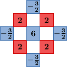
The demosaicking is implemented by convolution with a set of linear filters. There are eight different filters for interpolating the different color components at different locations. The filters are shown below.

G at red locations		G at blue locations
R at green locations in red rows		R at green locations in blue rows		R at blue locations
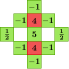B at green locations in red rows		B at green locations in blue rows		B at red locations
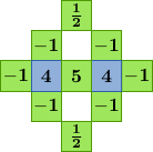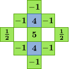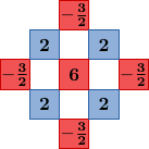The 5×5 linear filters. The coefficient values are scaled by 8.

For example, at a green pixel location in a red row, the red component is interpolated by

The filters can be implemented using integer arithmetic. Suppose that the input CFA data is given as a 2D integer array F(i,j), then the interpolation above can be implemented as

R(i,j) = ( F(i,j-2) + F(i,j+2)
           - 2*(F(i-1,j-1) + F(i+1,j-1) + F(i-2,j) + F(i+2,j) + F(i-1,j+1) + F(i+1,j+1))
           + 8*(F(i-1,j) + F(i+1,j))
           + 10*F(i,j) ) / 16

and the division by 16 can be efficiently implemented by bitshifting. The other filters are implemented similarly.

Implementation

This software includes the implementations of algorithms potentially linkable to patents. Various distribution terms apply. Some files are distributed under the terms of the simplified BSD license, some are for scientific and education use only.

• source code zip tar.gz
• online documentation

Please see the readme.html file or the online documentation for details.

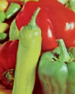
Examples

Considering its simplicity, the method works surprisingly well compared to more complicated methods. Aside from the bilinear interpolation, all other methods shown here are either nonlinear or use larger filter support.

Exact	Observed Image	Bilinear (PSNR 29.47)
Gunturk et al. [4] (PSNR 26.98)	Li [6] (PSNR 23.58)	Hamilton-Adams [2] (PSNR 29.17)
Zhang-Wu [7] (PSNR 28.94)	Buades et al. [9] (PSNR 29.11)	Malvar-He-Cutler (PSNR 29.66)

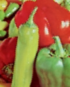Bilinear interpolation and Hamilton-Adams methods are also low-cost demosaicking methods, so it is interesting to compare particularly with them. The example below shows that Malvar-He-Cutler is visually sharper than bilinear, but not as sharp as Hamilton-Adams. This is because Hamilton-Adams uses a nonlinear interpolation strategy.

Exact	Observed Image	Bilinear (PSNR 25.61)
Hamilton-Adams [2] (PSNR 31.62)	Malvar-He-Cutler (PSNR 31.15)

This material is based upon work supported by the National Science Foundation under Award No. DMS-1004694. Any opinions, findings, and conclusions or recommendations expressed in this material are those of the author(s) and do not necessarily reflect the views of the National Science Foundation. Work partially supported by the MISS project of Centre National d'Etudes Spatiales, the Office of Naval Research under grant N00014-97-1-0839 and by the European Research Council, advanced grant “Twelve labours.”

image credits