mcm/FDS_MCM.c File Reference
Finite Difference Scheme for the Mean Curvature Motion. More...
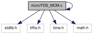
#include <stdlib.h>#include <tiffio.h>#include "io_tiff_routine.h"#include <time.h>#include <math.h>

Go to the source code of this file.
Defines | |
| #define | FATAL(MSG) |
| #define | INFO(MSG) |
| #define | DEBUG(MSG) |
Functions | |
| static void | heat (float *ptr_out, float *ptr_in, size_t n_col, int i, int i_prev, int i_next, int j, int j_prev, int j_next, float dt) |
| Computes one iteration of Heat Equation. | |
| static void | mcm (float *ptr_out, float *ptr_in, size_t n_row, size_t n_col, float dt, float t_g) |
| Computes one iteration of the Mean Curvature Motion. | |
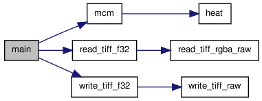
| int | main (int argc, char *argv[]) |
| Main function call. | |
Detailed Description
Finite Difference Scheme for the Mean Curvature Motion.
- Version:
- 1.3
requirements:
- ANSI C compiler
- libtiff
compilation:
- type "gcc FDS_MCM.c io_tiff_all.c -ltiff -o mcm.out" to obtain the executable file
- type "mcm.out" followed by the required arguments to run the executable file
usage: this programs requires 3 arguments written in the following order,
- argv[1] contains the normalized scale you want to reach
- argv[2] contains the name of the input file
- argv[3] contains the name of the output file
The normalized scale represents the scale  at which a circle with radius
  disappears. The number of iterations needed is linked to normalized scale and time step by the following formula:
![\[ n_{iter}= \frac{R^2}{2 \cdot dt} \]](form_1.png)
where  is the normalized scale,
  the time step and
  the number of iterations.
Definition in file FDS_MCM.c.
Define Documentation
| #define DEBUG | ( | MSG | ) |
| #define FATAL | ( | MSG | ) |
| #define INFO | ( | MSG | ) |
Function Documentation
| static void heat | ( | float * | ptr_out, | |
| float * | ptr_in, | |||
| size_t | n_col, | |||
| int | i, | |||
| int | i_prev, | |||
| int | i_next, | |||
| int | j, | |||
| int | j_prev, | |||
| int | j_next, | |||
| float | dt | |||
| ) | [static] |
Computes one iteration of Heat Equation.
This function applies the following Finite Difference Scheme for Heat Equation
![\[ u_{n+1} = u_n + dt \cdot \Delta u_n \]](form_4.png)
where the discrete laplacian  is given by
![\[ \Delta u_n = u_n(i+1,j) + u_n(i-1,j) + u_n(i,j+1) + u_n(i,j-1) - 4u_n(i,j) \]](form_6.png)
- Parameters:
-
[out] ptr_out pointer to the output array [in] ptr_in pointer to the input array [in] n_col number of columns i current row i_prev previous row i_next next row j current column j_prev previous column j_next next column [in] dt time step
Definition at line 138 of file FDS_MCM.c.

| int main | ( | int | argc, | |
| char * | argv[] | |||
| ) |
Main function call.
The program reads an image.tiff given as input, applies a Finite Difference Scheme for the Mean Curvature Motion at renormalized scale  , writes the result as a new image.tiff and returns it as output.
Definition at line 357 of file FDS_MCM.c.

| static void mcm | ( | float * | ptr_out, | |
| float * | ptr_in, | |||
| size_t | n_row, | |||
| size_t | n_col, | |||
| float | dt, | |||
| float | t_g | |||
| ) | [static] |
Computes one iteration of the Mean Curvature Motion.
This function applies a Finite Difference Scheme for the Mean Curvature Motion
![\[ u_t=|Du|curv(u) \]](form_7.png)
When  , we denote by
  the direction orthogonal to
  and by
  the angle between the
  positive semiaxis and the gradient. Since
![\[ u_{\xi\xi}=D^2u(\xi,\xi)=D^2u\Bigl(\frac{Du^{\perp}}{|Du|},\frac{Du^{\perp}} {|Du|}\Bigr)= \frac{1}{|Du|^2}D^2u(Du^{\perp},Du^{\perp})= |Du|curv(u) \]](form_13.png)
the continuous equation can be translated in the followig discrete version:
![\[ u_{n+1}(i,j)=u_n(i,j)+\Delta t (u_{\xi\xi})_n(i,j) \]](form_14.png)
For the numerical evaluation of  we adopt a linear finite difference scheme based on a
  stencil.
![\[ (u_{\xi \xi})_n(i,j)= \frac{1}{\Delta x^2}( \hspace{0.3em} -4\lambda_0 \cdot u_n(i,j) \hspace{0.3em} + \hspace{0.3em} \lambda_1 \cdot (u_n(i,j+1) + u_n(i,j-1)) \hspace{0.3em} + \hspace{0.3em} \lambda_2 \cdot (u_n(i+1,j) + u_n(i-1,j)) \hspace{0.3em} + \hspace{0.3em} \lambda_3 \cdot (u_n(i-1,j-1) +u_n(i+1,j+1)) \hspace{0.3em} + \hspace{0.3em} \lambda_4 \cdot (u_n(i-1,j+1) +u_n(i+1,j-1)) \hspace{0.3em}) \]](form_17.png)
The later can be rewritten in a more synthetic form, using a discrete convolution with a variable kernel 
![\[ u_{\xi\xi_n}=\frac{1}{\Delta x^2}\cdot (A \star u_n) \quad \mbox{where} \quad A=\Biggl(\begin{array}{ccc} \lambda_3(\theta) & \lambda_2(\theta) & \lambda_4(\theta) \\ \lambda_1(\theta) & -4\lambda_0(\theta) & \lambda_1(\theta) \\ \lambda_4(\theta) & \lambda_2(\theta) & \lambda_3(\theta) \end{array} \Biggr) \]](form_19.png)
We talk about  since the
  depend on the direction of
  and can be calculated either from
  and
and  or (as we do in the code to optimize the number of variables allocated) directly from the FDS of the partial derivatives
  and
and  .
.
![\[ \begin{array}{l} u_x= \displaystyle \frac{2\cdot (u(i,j+1) - u(i,j-1)) + u(i-1,j+1) - u(i-1,j-1) + u(i+1,j+1) - u(i+1,j-1)} {8\Delta x}= \displaystyle \frac{s_x}{8\Delta x} \\ \\ u_y= \displaystyle \frac{2\cdot (u(i+1,j) - u(i-1,j)) + u(i+1,j+1) - u(i-1,j+1) + u(i+1,j-1) - u(i-1,j-1)} {8\Delta x}= \displaystyle \frac{s_y}{8\Delta x} \\ \end{array} \]](form_27.png)
where we have denoted respectively by  and
and  the algebric sums at the numerator of
  and
and  .
.
With the choice  the following formulas hold for the
  :
:
![\[ \begin{array}{l} \lambda_0= \displaystyle \frac{1}{2} - \frac{s_x^2 \cdot s_y^2} {(s_x^2+s_y^2)^2} \\ \\ \lambda_1= 2\lambda_0 - \displaystyle \frac{s_x^2}{s_x^2+s_y^2} \\ \\ \lambda_2= 2\lambda_0 - \displaystyle \frac{s_y^2}{s_x^2+s_y^2} \\ \\ \lambda_3= -\lambda_0 +\displaystyle \frac{1}{2} \cdot \Bigl(1-\frac{s_x \cdot s_y} {s_x^2+s_y^2}\Bigr) \\ \\ \lambda_4= -\lambda_0 +\displaystyle \frac{1}{2} \cdot \Bigl(1+\frac{s_x \cdot s_y} {s_x^2+s_y^2}\Bigr) \end{array} \]](form_32.png)
Remember that the array representing the image is examinated as a matrix, i.e.  :
:  is the current row number and
  is the current column number. The infinitezimal increment
  is the pixel width and is set to
  .
.
At the borders, we symmetrize the image with respect to the axes  and
and  , i.e.
![\[ \begin{array}{l} u(-1,j) = u(0,j) \\ \\ u(n_{row},j) = u(n_{row}-1,j) \\ \\ u(i,-1) = u(i,0) \\ \\ u(i,n_{col}) = u(i,n_{col}-1) \end{array} \]](form_40.png)
All these speculations are based on the hypothesis that  . In fact
  , which means that, if
  , the Mean Curvature Motion is undefined and has no sense talking about
  or
or  . Numerically, even if the gradient is
  , but small in modulus, its direction becomes substantially random, because it will be driven by rounding and approximation errors.
These considerations bring us to replace  by half the laplacian, if
  is below a given threshold (experimentally set to
  ).
).
- Parameters:
-
[out] ptr_out pointer to the output array [in] ptr_in pointer to the input array [in] n_row number of rows [in] n_col number of columns [in] dt time step [in] t_g threshold for the gradient
Definition at line 281 of file FDS_MCM.c.


 1.6.3
1.6.3