Micro-Texture Synthesis by Phase Randomization

Bruno Galerne; Yann Gousseau; Jean-Michel Morel

doi:10.5201/ipol.2011.ggm_rpn

Bruno Galerne, Yann Gousseau, Jean-Michel Morel

→ BibTeX

@article{ipol.2011.ggm_rpn,
    title   = {{Micro-Texture Synthesis by Phase Randomization}},
    author  = {Galerne, Bruno and Gousseau, Yann and Morel, Jean-Michel},
    journal = {{Image Processing On Line}},
    volume  = {1},
    year    = {2011},
    doi     = {10.5201/ipol.2011.ggm_rpn},
}
% if your bibliography style doesn't support doi fields:
    note    = {\url{http://dx.doi.org/10.5201/ipol.2011.ggm_rpn}}

published: 2011-09-23
reference: Bruno Galerne, Yann Gousseau, and Jean-Michel Morel, Micro-Texture Synthesis by Phase Randomization, Image Processing On Line, 1 (2011). http://dx.doi.org/10.5201/ipol.2011.ggm_rpn

Communicated by Gabriel Peyré
Demo edited by Nicolas Limare

Bruno Galerne, galerne@cmla.ens-cachan.fr, CMLA, ENS Cachan, CNRS, UniverSud
Yann Gousseau, gousseau@enst.fr, LTCI CNRS, Télécom ParisTech
Jean-Michel Morel, morel@cmla.ens-cachan.fr, CMLA, ENS Cachan, CNRS, UniverSud

Overview

Context

This contribution is concerned with texture synthesis by example, the process of generating new texture images from a given sample. This field has witnessed an important number of key contributions over the last 15 years, see e.g. (ref. 2, 3, 4, 5). In (ref. 2), the texture is reconstructed by a Markov Random field model directly inspired from Shannon's famous English sentence reconstruction. Each incomplete patch of the image under construction is compared to all patches of the sample image. The closest patches in the sample permit to predict a new pixel value in the synthetic image. The iterative algorithm grows in that way a new image from a random seed, or even from the sample itself by extending its boundaries. The method of (ref. 3) is a significant technical improvement of the same basic ideas, where the shape of the incomplete patch is no more variable. These patch-based algorithms suffer, however, from several drawbacks pointed out by the authors themselves: the resulting image is sometimes strikingly good, but sometimes also its statistics do not match those of the input and the algorithm may even diverge toward poorly structured results. Unwanted periodicities can also occur, the algorithm having a strong tendency to produce verbatim copy of the input. The algorithms (ref. 4, 5), inspired from models of human texture perception (e.g. ref. 6) and from wavelet theory, learn the wavelet coefficients statistics from the sample and enforce them in the reconstructed image. In (ref. 4) this reconstruction deals only with wavelet coefficient histograms while in (ref. 5) the cross-correlation and autocorrelation statistics of the wavelet channels are also enforced. The final results, particularly those of (ref. 5), are absolutely striking. The process is nonetheless quite complex, its convergence not guaranteed, and color artifacts may also appear. In short, in spite of considerable progress, no present algorithm delivers a full reproduction of all textures, and it is still important to explore other ways, well adapted to this or that kind of texture.

Contribution

The Random Phase Noise (RPN) algorithm presented here, and first introduced in the paper (ref. 1), synthesizes a texture from an original image by simply randomizing its Fourier phase. It is able to reproduce textures which are characterized by their Fourier modulus, namely the random phase textures (or micro-textures). It is also able to create a random texture from any input image. It is in spirit quite close to the noise generators from computer graphics, see e.g. (ref. 7, 8).

The presented algorithm deals with color images. It is able to synthesize output textures with arbitrary sizes. The algorithm is definitely limited to a certain class of textures, but it has the following good properties, that are particularly useful for graphic applications and are not shared by, e.g., exemplar-based methods.

It is fast, since it basically only needs the computation of two FFTs.
It is perceptually stable: all the textures synthesized from the same input image are visually similar. In particular, it will never grow garbage.
It will never yield verbatim copy of the original.
It has no convergence issues.

References

1. Galerne, Y. Gousseau and J.-M. Morel, Random Phase Textures: Theory and Synthesis, IEEE Trans. on Image Processing, 2011. DOI:10.1109/TIP.2010.2052822, pdf of preprint.
1. 1. Efros and T. K. Leung, Texture Synthesis by Non-parametric Sampling, Proceedings of ICCV, 1999. DOI:10.1109/ICCV.1999.790383
L.-Y. Wei and M. Levoy, Fast Texture Synthesis using Tree-structured Vector Quantization, Proceedings of SIGGRAPH, 2000. DOI:10.1145/344779.345009
1. 1. Heeger and J. R. Bergen, Pyramid-based texture analysis/synthesis, Proceedings of SIGGRAPH, 1995. DOI:10.1145/218380.218446
1. Portilla and E. P. Simoncelli, A Parametric Texture Model Based on Joint Statistics of Complex Wavelet Coefficients, Int. Journal of Computer Vision, 2000. DOI:10.1023/A:1026553619983
1. Malik and P. Perona, Preattentive texture discrimination with early vision mechanisms, J. Opt. Soc. Am. A 7, 923-932, 1990. DOI:10.1364/JOSAA.7.000923
1. Perlin, An image synthesizer, Proceedings of SIGGRAPH, 1985. DOI:10.1145/325165.325247
1. 1. van Wijk, Spot noise texture synthesis for data visualization, Proceedings of SIGGRAPH, 1991. DOI:10.1145/127719.122751
1. Moisan, Periodic plus Smooth Image Decomposition, Journal of Mathematical Imaging and Vision, 2011. DOI:10.1007/s10851-010-0227-1

Online Demo: Try It!

An on-line demo of this algorithm is available.

The demo permits to upload a color texture sample and to replicate it with arbitrary size. Texture samples can be taken from existing databases, but to have still more realistic samples, you can extract them as homogeneous regions of a photograph, as shown below in What are micro-textures?

Source Code

An implementation is available for download. It is provided with an illustated html documentation:

Source code zip;
Illustrated documentation zip, online;

This code requires libpng, libfftw3 and getopt. It should compile on any system since it's only ANSI C. Compilation and usage instruction are included in the README.txt file of the archive zip.

The illustrated HTML documentation can be reproduced from the source code zip by using doxygen (see the README.txt file of the archive zip for details).

Algorithm

Basic RPN

By definition, the RPN of an image h is the random image obtained by adding a random phase θ to the Fourier phase of the image. By a random phase we mean a white noise image uniformly distributed over [-π,π] and that is constrained to be symmetric. Then the basic RPN algorithm consists in:

Computing a realization θ of a random phase.
Computing the discrete Fourier transform (DFT) $\hat{h}$ of h.
Adding the random phase:

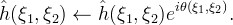
$\hat{h}(\xi_1,\xi_2) \leftarrow \hat{h}(\xi_1,\xi_2) e^{i\theta(\xi_1,\xi_2)}.$

Returning the inverse DFT of $\hat{h}$ .

Extension to Color Images

The RPN of an RGB color image h=(h_R, h_G, h_B) is obtained by adding the same random phase to the DFT of each color channel. More precisely, step 3. of the above basic RPN algorithm is replaced by

$\left(\hat{h}_R(\xi_1,\xi_2),\hat{h}_G(\xi_1,\xi_2),\hat{h}_B(\xi_1,\xi_2)\right) \leftarrow \left(\hat{h}_R(\xi_1,\xi_2),\hat{h}_G(\xi_1,\xi_2),\hat{h}_B(\xi_1,\xi_2)\right) e^{i\theta(\xi_1,\xi_2)}.$

Adding the same random phase to the original phases of each color channel preserves the phase displacements between channels. This is important as it permits to create new textures without creating false colors (see ref. 1).

Avoiding Artifacts Due to Non Periodicity

The RPN algorithm is based on the FFT and consequently the periodicity of the input image is a critical requirement. Indeed, as experiments show, randomizing the phase of an image which is not periodic creates strong artifacts consisting in highly contrasted horizontal and vertical waves. To avoid these artifacts the input image h is replaced by its periodic component p as defined by L. Moisan in (ref. 9).

The periodic component p is the unique solution of the problem

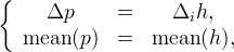
$\left\{ \begin{array}{ccc} \Delta p & = & \Delta_i h, \\ \operatorname{mean}(p) & = & \operatorname{mean}(h), \end{array} \right.$

where Δ is the usual discrete periodic Laplacian (each point has four neighbors) and $\Delta_i$ is the discrete Laplacian in the interior of the image domain (points at the border of the image have only three or two neighbors).

The periodic component p of h is computed using the classic FFT-based Poisson solver:

Compute the discrete Laplacian $\Delta_i h$ of h.
Compute the DFT $\widehat{\Delta_i h}$ of $\Delta_i h$ .
Compute the DFT $\hat{p}$ of p by inversing the discrete periodic Laplacian:

$\left\{ \begin{array}{ccc} \hat{p}(\xi_1,\xi_2) & = & \left(4-2\cos\left( \frac{2 \xi_1 \pi}{M} \right)-2\cos\left( \frac{2 \xi_2 \pi}{N}\right)\right)^{-1} \widehat{\Delta_i h}(\xi_1,\xi_2),\\ \hat{p}(0) & = & \sum_{(x,y)} h(x,y). \end{array} \right.$

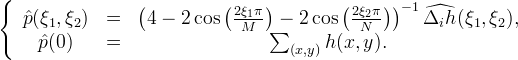
Compute p by inverse DFT.

Note that this procedure permits to compute the DFT $\hat{p}$ of p using only one call to the FFT algorithm. Let us also precise that computing the periodic component of a color image simply consists in computing the periodic component of each color channel.

Spot Extension Technique

An important issue in texture synthesis is to synthesize textures with arbitrary large size from a given sample.

A practical method solves this problem for RPN textures. This is done by extending the original texture sample into an equivalent spot having a larger size, and then by applying the basic RPN algorithm to this larger equivalent spot, as illustrated in the example below.

A texture image (left) and its corresponding extended spot (right)

Let us specify how the extended spot is computed. First, the periodic component of the original texture sample is computed and pasted in a large constant image equal to the mean of the sample, with a previous variance normalization. The obtained image is then multiplied by a smooth transition function in order to attenuate the discontinuities along the inner frame of the spot. On the interval [0,1], the smooth transition function $\varphi_\alpha$ is defined as follows: On [0,α] the function varies as the primitive of the standard $\mathcal{C}^{\infty}$ function

$t \mapsto \exp\left(-1/\left(1-(2t/\alpha -1)^2\right)\right),$

it is symmetrically defined on the interval [1-α,1] and it is constant to 1 on the inner interval [α,1-α]. Below are both a cross section and a gray-level representation of the smooth transition function used to attenuate the spot along the border of the image.

Smooth transition function used to attenuate the extended spot along the border of the image

In addition, in order to preserve the variance of the initial spot, the smooth function is normalized so that its L²-norm equals 1. The value of the parameter α is not a sensitive parameter. For all experiments as well as for the online demo the parameter α has been fixed to α=0.1. However α is an optional parameter of the downloadable source code.

Implementation

Our implementation consists in two distinct procedures: same size RPN and increased size RPN.

Same size RPN

The whole algorithm for synthesizing a RPN texture having the same size as the original image h consists in the following steps:

Compute the DFT $\hat{p}$ of the periodic component p of the input image h.
Compute a realization θ of a random phase.
Add the random phase θ to each color channel of $\hat{p}$ .
Return the inverse DFT of the phase randomized $\hat{p}$ .

Note that this algorithm only uses two calls to the FFT algorithm.

Increased size RPN

Compute the periodic component p of the input image h.
Extend the periodic component p into an equivalent spot of larger size using the spot extension technique described above.
Compute a random phase θ having the same size as the extended spot.
Compute the RPN in adding the random phase θ to the DFT of each color channel.

This procedure is computationally more expensive than for the "same size RPN". Indeed, it makes four calls of the FFT algorithm: two with the size of the original spot h for the computation of the periodic component p, and two with the larger output size for the phase randomization.

Micro-Textures

What are Micro-textures

When photographed, remote homogeneous areas made of thin, small, or semitransparent objects create homogeneous regions in images. The geometric features and colors of the constituents of the observed area are mixed, due to the blur inherent to image formation. The resulting image region is a micro-texture. Most homogeneous regions in any image should be micro-textures. The figure below shows an example. Five rectangles belonging to various homogeneous regions were picked in a high resolution landscape. These textures are displayed in pairs where the left is the original sub-image, and the right a simulation obtained by the RPN algorithm. With the exception of the clouds rectangle (which is obviously non-stationary), these samples and their simulated copies are usually considered perceptually equivalent by observers. Here pebbles, wet sand, and various types of waves are correctly simulated.

Some emulated textures taken from an high resolution landscape

Yet, not all homogeneous regions of an image are micro-textures. See below many examples, and the failure catalog as well.

Micro-textures and Macro-textures

Many images or image parts usually termed textures do not fit to the micro-texture requisites. Typically, periodic patterns with big visible elements, such as brick walls, are not micro-textures. More generally, textures whose building elements are spatially organized, such as the branches of a tree, are not micro-textures. Yet, each textured object has a critical distance at which it becomes a micro-texture. For instance, tiles at a close distance are a macro-texture, and are not amenable to phase randomization. The smaller tiles on roofs photographed at some distance can instead be emulated.

Microtextures: tiled roofs

Samples

RPN

Tiles from roof 1

Tiles from roof 1 emulated by RPN

Tiles from roof 2

Tiles from roof 2 emulated by RPN

A macro-texture: tiles at short range

RPN failure to simulate a macro-texture

Examples

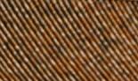
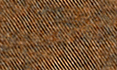
Below are some examples of satisfyingly well reproduced textures of wood, wall, fabric, and paint. Note that one has to click on the examples to see their real size. See also the failure catalog for examples which are not well reproduced.

Wood

Wood samples must be homogeneous in direction to be correctly emulated by RPN. Wood samples with knots or other conspicuous patterns fall logically in the failure catalog.

Wood sample	RPN simulation

More Wood Examples

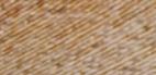
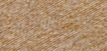
Fabric

Fabric sample	RPN simulation

More Fabric Examples

Walls

Wall sample	RPN simulation

More Wall Examples

Paint

Paint sample	RPN simulation

More Paint Examples

Failure Catalog

Most failures are macro-textures. For instance:

textures containing periodic geometric patterns with large period,
textures containing strong edges, such as cracks in bark,
textures containing definite shapes, such as knots in wood or fruit or visible leaves in foliage,
strictly periodic patterns, even with small period, where phase shifts cause aliasing effects,
failure also occurs when the sample texture contains different dominant directions in different areas. Then these directions are mixed by the random sampler.

Macro-texture sample	RPN simulation

More Failure Examples

image credits