amss/FDS_AMSS.c File Reference
Finite Difference Scheme for the Affine Morphological Scale Space. More...
#include <stdlib.h>#include <tiffio.h>#include <time.h>#include <math.h>#include "io_tiff_routine.h"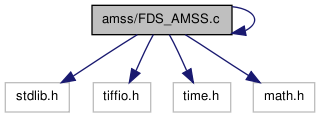

Go to the source code of this file.
Defines | |
| #define | FATAL(MSG) |
| #define | INFO(MSG) |
| #define | DEBUG(MSG) |
Functions | |
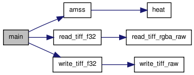
| static void | heat (float *ptr_out, float *ptr_in, size_t n_col, int i, int i_prev, int i_next, int j, int j_prev, int j_next, float dt) |
| Computes one iteration of Heat Equation. | |
| static void | amss (float *ptr_out, float *ptr_in, size_t n_row, size_t n_col, float dt, float t_g) |
| Computes one iteration of the Affine Morphological Scale Space. | |
| int | main (int argc, char *argv[]) |
| main function call | |
Detailed Description
Finite Difference Scheme for the Affine Morphological Scale Space.
- Version:
- 1.3
requirements:
- ANSI C compiler
- libtiff
compilation:
- type "gcc FDS_AMSS.c io_tiff_all.c -ltiff -o amss.out" to obtain the executable file
- type "amss.out" followed by the required arguments to run the executable file
usage: this programs requires 3 arguments written in the following order,
- argv[1] contains the normalized scale you want to reach
- argv[2] contains the name of the input file
- argv[3] contains the name of the output file
The normalized scale represents the scale  at which a circle with radius disappears. The number of iterations needed is linked to normalized scale and time step by the following formula:
![\[ n_{iter}= \frac {3}{4 \cdot dt} R^{\frac{4}{3}} \]](form_1.png)
where is the normalized scale,  the time step and
  the number of iterations.
Definition in file FDS_AMSS.c.
Define Documentation
| #define DEBUG | ( | MSG | ) |
do {\
        if (debug_flag)\
            fprintf(stderr, __FILE__ ":%03i " MSG "\n", __LINE__);\
    } while (0);
print a debug message, with detailed information
Definition at line 95 of file FDS_AMSS.c.
| #define FATAL | ( | MSG | ) |
do {\
          fprintf(stderr, MSG "\n");\
        abort();\
        } while (0);
print a message and abort the execution
Definition at line 82 of file FDS_AMSS.c.
| #define INFO | ( | MSG | ) |
do {\
        fprintf(stderr, MSG "\n");\
    } while (0);
print an info message
Definition at line 89 of file FDS_AMSS.c.
Function Documentation
| static void amss | ( | float * | ptr_out, | |
| float * | ptr_in, | |||
| size_t | n_row, | |||
| size_t | n_col, | |||
| float | dt, | |||
| float | t_g | |||
| ) | [static] |
Computes one iteration of the Affine Morphological Scale Space.
This function applies a Finite Difference Scheme for Affine Curvature Motion
![\[ u_t=|Du|(curv(u))^{\frac{1}{3}}= (|Du|^3 curv(u))^{\frac{1}{3}} \]](form_7.png)
Similarly to MCM, when  , we denote by
  the direction orthogonal to
  and by
  the angle between the
  positive semiaxis and the gradient. Hence
![\[ u_{\xi\xi}=D^2u(\xi,\xi)=D^2u\Bigl(\frac{Du^{\perp}}{|Du|},\frac{Du^{\perp}} {|Du|}\Bigr)= \frac{1}{|Du|^2}D^2u(Du^{\perp},Du^{\perp})= |Du|curv(u) \]](form_13.png)
and the continuous equation can be translated in this discrete version:
![\[ u_{n+1}(i,j)= u_n(i,j) + + \Delta t \cdot (|Du_n|^2 (u_{\xi\xi})_n)^{\frac{1}{3}}(i,j) \]](form_14.png)
As regards the numerical evaluation of  , we adopt a linear finite difference scheme based on a
  stencil.
![\[ |Du_n|^2 (u_{\xi\xi})_n (i,j)=\frac{1}{\Delta x^2}( \hspace{0.3em} -4\eta_0 \cdot u_n(i,j)\hspace{0.3em} + \hspace{0.3em} \eta_1 \cdot (u_n(i,j+1) + u_n(i,j-1)) \hspace{0.3em} + \hspace{0.3em} \eta_2 \cdot (u_n(i+1,j) + u_n(i-1,j)) \hspace{0.3em} + \hspace{0.3em} \eta_3 \cdot (u_n(i-1,j-1) + u_n(i+1,j+1)) \hspace{0.3em} + \hspace{0.3em} \eta_4 \cdot (u_n(i-1,j+1) + u_n(i+1,j-1)) \hspace{0.3em}) \]](form_17.png)
which can be rewritten in a more synthetic form, using a discrete convolution with a variable kernel 
![\[ |Du_n|^2 (u_{\xi\xi})_n=\frac{1}{\Delta x^2}\cdot (B \star u_n) \quad \mbox{where} \quad B=\Biggl( \begin{array}{ccc} \eta_3(\theta) & \eta_2(\theta) & \eta_4(\theta) \\ \eta_1(\theta) & -4\eta_0(\theta) & \eta_1(\theta) \\ \eta_4(\theta) & \eta_2(\theta) & \eta_3(\theta) \end{array} \Biggr) \]](form_19.png)
We talk about  since the
  depend on the direction of
  and can be calculated directly from the FDS of the partial derivatives
  and
and  .
.
![\[ \begin{array}{l} u_x= \displaystyle \frac{2\cdot (u(i,j+1) - u(i,j-1)) + u(i-1,j+1) - u(i-1,j-1) + u(i+1,j+1) - u(i+1,j-1)} {8\Delta x}= \displaystyle \frac{s_x}{8\Delta x} \\ \\ u_y= \displaystyle \frac{2\cdot (u(i+1,j) - u(i-1,j)) + u(i+1,j+1) - u(i-1,j+1) + u(i+1,j-1) - u(i-1,j-1)} {8\Delta x}= \displaystyle \frac{s_y}{8\Delta x} \\ \end{array} \]](form_25.png)
where we have denoted respectively by  and
and  the algebric sums at the numerator of and .
A very similar procedure is followed if we want to obtain an algorithm for MCM. The only difference is that for the Mean Curvature Motion we must discretize only  , which can be seen again as the result of a convolution with a discrete kernel
  :
:
![\[ u_{\xi\xi_n}=\frac{1}{\Delta x^2}\cdot (A \star u_n) \quad \mbox{where} \quad A=\Biggl(\begin{array}{ccc} \lambda_3(\theta) & \lambda_2(\theta) & \lambda_4(\theta) \\ \lambda_1(\theta) & -4\lambda_0(\theta) & \lambda_1(\theta) \\ \lambda_4(\theta) & \lambda_2(\theta) & \lambda_3(\theta) \end{array} \Biggr) \]](form_30.png)
Thus the choice of the can be reduced to that of the  , since
  for
for  . Experiments have shown that if we take
  , i.e. the same value used in MCM, the best results as regards stability are achieved. Therefore the following formulas are actually adopted in the algorithm:
![\[ \begin{array}{l} \eta_0=\displaystyle\frac{1}{2} \cdot (u_x^2+u_y^2)-\frac{u_x^2 \cdot u_y^2} {u_x^2+u_y^2} \\ \\ \eta_1= 2\eta_0 - u_x^2 \\ \\ \eta_2= 2\eta_0 - u_y^2 \\ \\ \eta_3= -\eta_0 + \displaystyle \frac{1}{2} \cdot (u_x^2 + u_y^2 - u_x \cdot u_y) \\ \\ \eta_4= -\eta_0 + \displaystyle \frac{1}{2} \cdot (u_x^2 + u_y^2 + u_x \cdot u_y) \end{array} \]](form_35.png)
Remember that the array representing the image is examinated as a matrix, i.e.  :
:  is the current row number and
  is the current column number. The infinitezimal
  is the pixel width and is set to
  .
.
On the border, we symmetrize the image with respect to the axes  and
and  , i.e.
![\[ \begin{array}{l} u(-1,j) = u(0,j) \\ \\ u(n_{row},j) = u(n_{row}-1,j) \\ \\ u(i,-1) = u(i,0) \\ \\ u(i,n_{col}) = u(i,n_{col}-1) \end{array} \]](form_43.png)
From a theorical point of view, even if we divide by the gradient, there is no need to apply Heat Equation when  .
.
In fact  and, if
  the Affine Morphological Scale Space is well defined. In addition even
  and consequently all the are well defined in the limit, since
  .
.
However rounding and approximation errors lead us to replace AMSS with Heat Equation when the gradient is below a threshold (experimentally set to  for the first iteration and then reduced to for the next ones).
- Parameters:
-
[out] ptr_out pointer to the output array [in] ptr_in pointer to the input array [in] n_row number of rows [in] n_col number of columns [in] dt time step [in] t_g threshold for the gradient
Definition at line 301 of file FDS_AMSS.c.


| static void heat | ( | float * | ptr_out, | |
| float * | ptr_in, | |||
| size_t | n_col, | |||
| int | i, | |||
| int | i_prev, | |||
| int | i_next, | |||
| int | j, | |||
| int | j_prev, | |||
| int | j_next, | |||
| float | dt | |||
| ) | [static] |
Computes one iteration of Heat Equation.
This function applies the following Finite Difference Scheme for Heat Equation
![\[ u_{n+1} = u_n + dt \cdot \Delta u_n \]](form_4.png)
where the discrete laplacian  is given by
![\[ \Delta u_n = u_n(i+1,j) + u_n(i-1,j) + u_n(i,j+1) + u_n(i,j-1) - 4u_n(i,j) \]](form_6.png)
- Parameters:
-
[out] ptr_out pointer to the output array [in] ptr_in pointer to the input array [in] n_col number of columns i current row i_prev previous row i_next next row j current column j_prev previous column j_next next column [in] dt time step
Definition at line 135 of file FDS_AMSS.c.

| int main | ( | int | argc, | |
| char * | argv[] | |||
| ) |
main function call
The program reads an image.tiff given as input, applies a Finite Difference Scheme for the Affine Morphological Scale Space at renormalized scale , writes the result as a new image.tiff and returns it as output.
Definition at line 380 of file FDS_AMSS.c.